Download
1 / 27
280 likes | 320 Views
Understand the concept of algorithms through formal models like Turing Machines. Learn why studying formal models is crucial and how they impact mathematical problem-solving. Explore Hilbert’s 10th problem and the Church-Turing Thesis. Delve into the distinction between decidable and recursively enumerable languages. Enhance your knowledge of algorithms and their role in computation theory.

E N D
Formal Models of Computation What’s an algorithm?
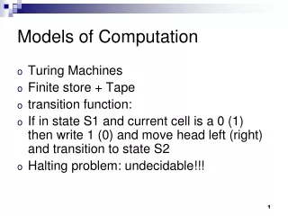
Formal models of computation • We briefly examined the lambda calculus, a formal model underlying Haskell • We shall explore another model of computation (called the imperative model), which underlies languages such as FORTRAN, PASCAL, C, JAVA etc: • The name of this model: Turing Machines (TMs) Why study formal models (instead of only specific implementations)? formal models of computation
“Formal models of computation” make precise what it means for a problem to be solvable by means of computation • Which problems are “computable” in a given type of programming language? • Best addressed by looking at a small prog. Language • The answer does not depend on the type of programming language (functional / logical / imperative): they are all equivalent • Church’s Thesis: they all formalise the notion of an algorithm • This course focusses on the imperative model (i.e., Turing Machines) formal models of computation
The Definition of Algorithm • Informally, an algorithm is • A sequence of instructions to carry out some task • A procedure or a “recipe” • Algorithms have had a long history in maths: • Find prime numbers • Find greatest common divisors (Euclid, ca. 300 b.C.!) • “Algorithm” was not defined until recently (1900’s) • Before that, people had an intuitive idea of algorithm • This intuitive notion was insufficient to gain a better understanding of algorithms formal models of computation
Algorithms in mathematics • Algorithms have had a long history in maths: • Find prime numbers • Find greatest common divisors (Euclid, ca. 300 b.C.!) • Mathematicians had an intuitive idea of algorithm • This intuitive notion was insufficient for proving things (e.g. for proving that a given problem cannot be solved by any algorithm) • Next: how the precise notion of algorithm was crucial to an important mathematical problem… formal models of computation
Hilbert’s Problems • David Hilbert gave a lecture • 1900 • Int’l Congress of Mathematicians, Paris • Proposal of 23 mathematical problems • Challenges for the coming century • 10th problem concerned algorithms • Before we talk about Hilbert’s 10th problem, let’s briefly discuss polynomials… formal models of computation
Polynomials • A polynomial is a sum of terms, where each term is a product of variables (which may be exponentiated by a natural number) and a constant called a coefficient • For example: 6x3yz2 + 3xy2 – x3 – 10 • A root of a polynomial • Assignment of values to variables so the polynomial is 0 • For example, if x = 5, y = 3 and z = 0, then (653302) + (3532) – 53 – 10 = 0 • This is an integral root: all variables assigned integers • Some polynomials have an integral root, some do not • x2 - 4 has integral root • x2 - 3 has no integral root formal models of computation
Hilbert’s 10th Problem • Devise an algorithm that tests if a polynomial has an integral root • Hilbert wrote “a process according to which it can be determined by a finite number of operations” • Hilbert assumed such an algorithm existed: we only need to find it! • We now know no algorithm exists for this task • It is algorithmically unsolvable: not computable • Impossible to conclude this with only an intuitive notion of algorithm! • Proving that an algorithm does not exist requires a clear definition of algorithm • Hilbert’s 10th Problem had to wait for this definition… formal models of computation
Church-Turing Thesis • The definition of algorithm came in 1936 • Papers by Alonzo Church and Alan Turing • Church proposed the -Calculus • Turing proposed Turing MachinesAutomata that are more powerful than FSAs (details to follow!) • These two definitions were shown to be equivalent, giving rise to the Church-Turing thesis • Thesis enabled a solution of Hilbert’s 10th problem • Matijasevic (1970) showed no such algorithm exists formal models of computation
Decidable versus Recursively Enumerable • A language L is called Recursively Enumerable iff there exists an algorithm that says YES to PRECISELY all the elements of L • It says YES to all the elements of L • It does not say YES to anything else • If x is not an element of the language then there are two possibilities: • The algorithm says NO to x • The algorithm does not find an answer formal models of computation
Turing-Recognisable Languages (Cont’d) • We prefer algorithms that always find an answer • They are called deciders • A language for which there exists a decider is called decidable. (We also say: the problem is decidable) • A decider decides the language consisting of all the strings to which it says YES • A decider for a language L answers every question of the form “Is this string a member of L?” in finite time • Algorithms that are not deciders keep you guessing on some strings • We shall soon see how these ideas pan out in connection with Turing Machines • First, Hilbert’s 10th problem formal models of computation
Hilbert’s 10th Problem as a formal language • Consider the set D = {p |p is a polynomial with an integral root} • Is Ddecidable? • Is there an algorithm that decides it? • The answer is NO! • However, D is Recursively Enumerable • To prove this, all we need to do is to supply an algorithm that “does the deed”: • The algorithm will halt if we input a polynomial that belongs to D, but it may loop if the polynomial does not belong to D formal models of computation
A simpler version of the 10th Problem Polynomials with only one variable: 4x3 – 2x2 + x – 7 D1={p |p is a polynomialover x withanintegralroot} An algorithm for D1: M1 = “The input is a polynomial p over x. 1. Evaluate p with x set successively to the values 0, 1, -1, 2, -2, 3, -3, … If at any point the polynomial evaluates to 0, say yes!” formal models of computation
A simpler version (Cont’d) • If p has an integral root, M1 will eventually find the root and accept p • If p does not have an integral root, M1 will run forever! • It’s like the problem of determining (e.g. in Haskell) whether a given infinite list contains 0. formal models of computation
A simpler version (Cont’d) • For the multivariable case, a similar algorithm M • M goes through all possible integer values for each variable of the polynomial… • Both M and M1 are algorithms but not deciders • Matijasevic showed 10th problem has no decider • This proof is omitted here. (But we shall prove another non-computability result later.) formal models of computation
Aside: Converting M1 into a Decider • The case with only 1 variable is decidable • We can convert M1 into a decider: • One can prove that the root x must lie between the values • k (cmax /c1 ) where k is the number of terms in the polynomial cmax is the coefficient with largest absolute value c1is the coefficient of the highest order term • We only have to try a finite number of values of x • If a root is not found within bounds, the machine rejects • Matijasevic: impossible to calculate bounds for multivariable polynomials. formal models of computation
TMs vs. Algorithms • Our focus is on algorithms • But it will help to have a more concrete idea of what an algorithm is • FSAs can be seen as algorithms, because they tell us which strings are elements of a language • However, FSAs do not allow us to do all the things that algorithms can do • Turing Machines (TMs) are much stronger automata • They are seen as faithful models for algorithms • This is Church’s thesis formal models of computation
“Philosophical” questions about Algorithms • Is an algorithm that’s not a decider (because on some inputs it does not terminate) really an algorithm? • Standard answer: yes. See the algorithm M1 above. • Is an algorithm that never terminates an algorithm? • Standard answer: yes. See Haskell’s definitions of the sequence of all Prime numbers. (Slides on Haskell.) Think of lambda terms that do not have a normal form. • Can an algorithm be stochastic? • Standard answer: yes. Think of nondeterministic FSAs. TMs can also be deterministic, and these TMs are generally thought of as algorithms • You may have different ideas, and they could be studied as well. formal models of computation
Uncomputable problems • We saw: If the answer to a yes/no problem can always be computed in finite time then the problem is called decidable • A more general term is “computable”: if the answer to a problem can always be computed in finite time then the problem called computable formal models of computation
Uncomputable problems • We saw: Computability is about what can be computed at all (in finite time) • Before going into computability, let’s look at what can be computed in a given programming language • First let’s prove in the abstract that some problems cannot be programmed in Haskell • The same method could be employed to show that some problems cannot be programmed in JAVA, etc. • We will employ the same method to show that some problems cannot be programmed in a TM formal models of computation
Theorem: some problems are not computable in Haskell Outline of proof: 1. There are uncountably many problems 2. There are countably many Haskell (JAVA, etc) programs 3. Conclusion: • Some problems cannot be programmed in Haskell (JAVA, etc.) Let’s look at this argument in more detail formal models of computation
First: There are countably many Haskell programs • Each Haskell program consists of a finite number of characters (the characters in the functions) • Each character is chosen from a finite set ( the set {a,b,…,z, A,B,..,Z, 0,1,2,..,9,’,’,(,),[,],:,.,|,^,&&,*,+,-,space} ) • So the set of Haskell programs can be enumerated • Enumerate all programs of length 1 character (if these exist), • Enumerate all programs of length 2 characters (if these exist), • … etc. Much like enumerating all rational numbers! • Discard all strings that do not make a wellformed Haskell program • The result is infinite but countable (like N) (“countably infinite”) formal models of computation
NB Our enumeration may contain functions that do not terminate (e.g., f may defined as f), so if you like (and if you can) you can discard these too • this will make the resulting set even smaller,so it does not affect our proof • The same argument shows that there are only countably many possible • JAVA programs • web pages • novels • ... • This is because each of these has a finite alphabeth and a finite (though unlimited!) length formal models of computation
Second: There are uncountably many problems/languages This is most easily shown by focussing on a particular class of problems. For example, • Consider all functions f :: Int -> IntEach defines a language of 3-tuples. For example (f1,x,y) iff f1(x)=y • The number of functions of this type is uncountable.Prove this using Cantor’s diagonal argument: Try to enumerate all functions fi; each fi(j) is defined for every integer j. Define a new function g as g(j)=fj+1.g cannot be an element of the enumeration. formal models of computation
Uncountably many f :: Int -> Int 1 2 3 4 5 6 7 8 ... f1 . f2 . f3 . f4 . ... g differs from f1 on the argument 1 g differs from f2 on the argument 2 ... etc. So: g is not in the enumeration! formal models of computation
Where we are now • You’ve seen a very abstract proof that some problems cannot be programmed in Haskell. • More specifically, you’ve seen that some functions f :: Int Int cannot be programmed in Haskell • But we haven’t shown you a concrete example (e.g., a concrete problem for which there is no Haskell program). • Is this a limitation of Haskell (JAVA,..)? No: We’ll • Introduce TMs • Argue that TMs can solve any computable problem • Show that TMs can’t program all programs formal models of computation
Reading List • Introduction to the Theory of Computation. Michael Sipser. PWS Publishing Co., USA, 1997. (A 2nd Edition has recently been published). Chapter 3. • Algorithmics: The Spirit of Computing. 3rd Edition. David Harel with Yishai Feldman. Addison-Wesley, USA, 2004. Chapter 9. formal models of computation