Download
1 / 18
210 likes | 444 Views
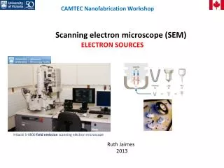
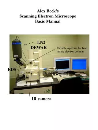
Alex Beck’s Scanning Electron Microscope Basic Manual. LN2 DEWAR. Variable Aperture for fine tuning electron column. EDS. IR camera. Table of Contents. Page # Cover Table of Contents Sample Stage Determining Atomic Number Field of Focus Vacuum Systems Electron Gun

E N D
Alex Beck’s Scanning Electron Microscope Basic Manual LN2 DEWAR Variable Aperture for fine tuning electron column EDS IR camera
Table of Contents • Page # • Cover • Table of Contents • Sample Stage • Determining Atomic Number • Field of Focus • Vacuum Systems • Electron Gun • Column Environment • Beam Sample Interaction • Electron Emission • Backscattered and Auger Electrons • SEM images • Energy Dispersive Spectrometer • EDS signal processing • SEM mapping • Preparing Sample • Photography • Quantitative EDS analysis
MOTORIZED PROGRAMABLE SAMPLE STAGE X-move Left to right on Screen Y-move Top to bottom on Screen Z-move Vertical Motion up and down Controls Working Distance. 41/2 mm minimum Tilt Tilts toward ET Detector only Rotate 360 degrees on sample axis Once Door is shut, activate ruffing pump to remove majority of air. Activate Turbomolecular / oil diffusion pump to remove more air. Once air pressure inside SEM falls below 10^-5 torr, turn on electron stream, and begin analysis.
3 SEPARATE INSTRUMENTS for determining atomic number: Scanning Electron Microscope SEM Base Platform for determining atomic number: : Energy Dispersive X-ray Spectrometer EDS Wave Dispersive X-ray Spectrometer WDS: nλ = 2 d Sin Θ Sin -1λ Char = Θ [set Detector] 2 d The SEM is for Imaging Surface Features and Topography SE Depth of Field Focus Composition: At. # and Shadow BSE Cathodlumniescence Chemical Variation The EDS is for Chemical Analysis Qualitative and Quantitative Analyses Point Analysis Line Analysis Area Analysis Elemental Mapping of Area
WHY SEM WORKS BETTER THAN OPTICAL MICROSCOPE Wavelength of Visible Light: Violet 400 nm to Red 750 nm wavelength DeBroglie Equation: λ = h/mv h = Planck’s Constant m = mass v = velocity For an electron wavelength this becomes: λ = 1.23/Voltage At 10 Kv acceleration voltage: 0.0123 nm wavelength At 30 Kv acceleration voltage: 0.0071 nm wavelength Optical field of focus: SEM field of focus:
SEM - Sub Component Systems Vacuum Systems Electron Gun Column Environment Chamber Environment Stage Detectors Beam - Sample Interaction Software SEM VACUUM SYSTEMS Mechanical Pump: [ 10 -3 torr] 760 mm Hg Roughing Pump Backing Pump Vapor Pump: Oil Diffusion Pump 10 –5 10 –6 torr Turbo Molecular Pump 10 -7 torr
The Electron Gun: Supplies electrons under variable acceleration voltage [ 1000 to 30,000 volts] Wehnelt Assembage Wehnelt Cylinder Filament Wehnelt Grid Anode Plate Filament Saturation Electron Emission False Peak Filament Current
THE COLUMN ENVIRONMENT Condensing Lenses (Electromagnetic) Controls “Spot Size” [Probe Current] Final Lens (Electromagnetic) Apertures: Fixed and Variable Scanning Coils: Electromagnetic Stigmator Coils: Electromagnetic fixes Astigmatism in beam shape Magnetic Lenses can become fixed on certain settings and must be degaussed, every once in a while to eliminate hysteresis memory, which can cause beam misalignment and blurry images. This effect is most pronounced when beam properties are changed, and magnetic field is realigned.
BEAM - SAM PLE INTERACTION Secondary Electrons (< 50 volts) SE Inelastic Collisions - 95% of electron population Back Scatter Electrons (5 - 30 Kev) BSE Elastic Collisions - 5% of electron Population Characteristic X-rays: Kalpha, K beta, etc. Bremstrahlung [X-ray Continuum - Breaking Radiation] Auger Electrons : Low Energy, top 1nm Cathodluminescence: : visible light Heat Volume of Excitation 10Kv Monte Carlo simulation of interaction volume with changing beam current 20Kv 30 Kv
Electron Population EVERHART - THORNLEY DETECTOR Secondary Electrons Imaging 1960
BACK SCATTER DETECTOR - Centarus Detector Annular Shape Solid state scintillation detector Directly above Sample and just below the Pole Piece Responds to electrons with several Kev and higher. Images appear without angular light perspective. Quad Detectors can correct this artificially Responds to Atomic Number Auger Electrons Low energy Only come from around top 1nm Require Auger Electron detector, somewhat new and expensive
BSE Image BSE Image SE Image BSE Image
is organic and very fragile, requires uniform pressure on both of its sides. 3.8 ev per hole-e
Energy Dispersive Spectrometer - EDS Artifact Signals - Signal Processing Summation Peaks: Produced by extremely high count rates. Small peak appears at exactly twice the ev value of a major peak. Two counts come in so fast that they are counted as one by the pulse Processor (50 nsec recovery) Example: Al = 1.49 Kev. 2 Al = 2.98 Kev Silicon Escape Peak : An incoming photoelectron causes the Si detector to emit a characterisitic 1.74 Kev Kalpha X-ray. If this X-ray escapes the system before being absorbed, it will take that energy away, and a small peak will appear at exactly 1.74 Kev LESS than some major peak ZAF CORRECTIONS Z = Atomic Number: Larger size atoms will produce more X-rays than smaller A = Absorbence of specific X- rays generated by one element by another. F = Fluorescence: X-ray emission induced by emission of other atoms. EDS MAPPING, with user defined color coding. Takes a long time to scan maps even at lower resolutions.
BSE SE CL CL MAP MAP
Preparing Sample Samples can be placed into SEM naked, but are normally mounted in Epoxy. Any Sample to be placed in SEM must either be conducting all the way through or be sputtered with an extremely thin conductive coating, usually gold or carbon. This is important as negation of conduction through or around sample results in build up of charge which repels other electrons and disrupts any analysis. Samples are normally prepared in a cylindrical epoxy mold. Too make mold place sample at bottom of container and pour in epoxy solution. Once epoxy has dried, remove mold from container. To grind mold down to sample use a very low grit sand paper, of for example 240. Use Buchler 1,000 Minimet Polishing, or equivalent. After sample is exposed wash sample and hands thoroughly to make sure no grains survive to a finer grit. Use an ultrasonic cleaner for approximately 10 minutes to shake out any further grains. Grind mold at higher grit ex. 320, then repeat above two steps. Apply even higher grit ex. 600, then repeat above two steps. Grind mold with 6 micrometer diamond solution apply same ultra sonic cleaning. Polish mold with .05 micrometer diamond solution, and wash. Just look at that mirror shine as you attach the mold to a mound with conducting carbon strips which both hold the mold in place and provide conduction to ground. Use sputter coater to coat mold with conductor. Place sample in SEM and begin analysis.
Photography Keep voltage around 20 kV Low magnification images usually have magnification less than 5,000X, with less concern for beam sample interactions. Long working distance normally around 20-30mm. Moderate to large spot size 200-300 notwithstanding. Higher magnification up to 100,000X, lessens depth of field and vice versa. Resolution is vital and should always be maximized. These are a few ways to increase resolution: Short working distance, 10-15mm NO LESS. Small spot size 100 or less. Small variable aperture. Use of Stigmater very important.
Quantitative EDS data analysis For optimal EDS analysis sample should be highly polished. 25V, 15 mm working distance, 400 spot size. Standardize beam to Cu standard that you place on sample mount. Processing time 5- 6 (slow), or 3-4 (fast) Dead time is when EDS is overwhelmed with data. Dead time must occupy less than 1/3 of time, or else recalibrate voltage and spot size. Aztec software user-friendly quick and easy, however lacks finer intricacies and extra functionality. Inca software is more professional and accurate and has a wide assortment of advanced features including color coded elemental mapping.