Sampling Distribution Models
80 likes | 99 Views
Understand the sampling distribution of loan payment proportions in a bank scenario, calculate mean and standard deviation, discuss underlying assumptions, and determine the probability of non-timely payments exceeding 10%. Clarify conditions for using the Normal model, considering sample size, population skewness, and the Central Limit Theorem. Illustrate with examples including coin toss experiments and sampling distribution models. In-depth examination of sampling distribution principles in statistics.

Sampling Distribution Models
E N D
Presentation Transcript
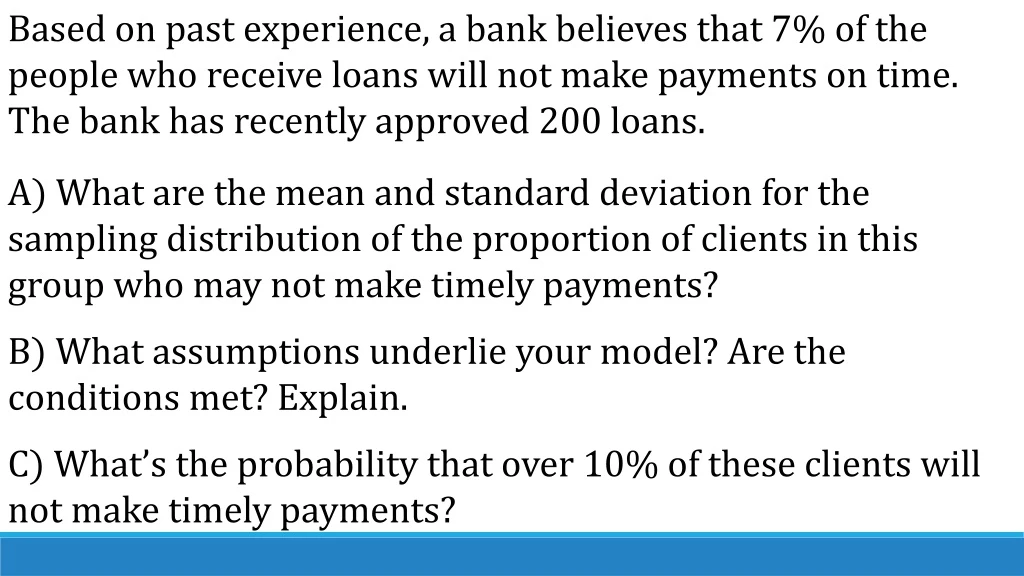
Based on past experience, a bank believes that 7% of the people who receive loans will not make payments on time. The bank has recently approved 200 loans. A) What are the mean and standard deviation for the sampling distribution of the proportion of clients in this group who may not make timely payments? B) What assumptions underlie your model? Are the conditions met? Explain. C) What’s the probability that over 10% of these clients will not make timely payments?
Sampling Distribution Models Chapter 18 Part 3
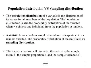
Sampling Distribution Models • Don’t confuse the sampling distribution with the distribution of the sample. • Watch out for skewed populations. The CLT assures us that we can use the Normal model for the sampling distributions, but the sample sizes will need to be larger if the population is skewed. A rule of thumb is to have sample size of at least 30.
We use the sample size to determine the standard deviation for the sampling distribution. Since n is in the denominator of the formula, the bigger the n, the smaller the standard deviation. Read pages 427 & 428
Example: In a large class of introductory Statistics, the professor has each person toss a coin 16 times and calculate the proportion of tosses that were heads. The students report their results, and the professor plots a histogram of these several proportions. What shape would you expect the histogram to be? Why? Where do you expect the histogram to be centered? How much variability would you expect among these proportions? Explain why a Normal model should not be used here. Symmetric. The sample size is small, but it is equally probably to get heads as it is to get tails. 0.5 because that is the probability of flipping a coin and landing on heads It does not meet the conditions since np = .5(16) = 8 and therefore np < 10.
Example: In a large class of introductory Statistics, the professor has each person toss a coin 26 times and calculate the proportion of tosses that were heads. a) Describe the sampling distribution using the 68-95-99.7 Rule. b) Confirm that you can use a Normal model here. c) The number of tosses is increased to 64. Draw and label the sampling distribution model. d) Explain how the sampling distribution changes as the number of tosses increases. Mean = 0.5, SD ≈ 0.1; 68% of sampling proportions are expected to be between 0.4 and 0.6; 95% are expected to be between 0.3 and 0.7; 99.7% are expected to be between 0.2 and 0.8 np = 13, nq = 13, and coin flips are independent N(0.5, 0.0625) As n increases, the standard deviation decreases. The distribution will still be symmetric, but less spread out (taller and more narrow).
Investigative Task: Simulated Coins Find a partner and find a calculator!
Today’s Assignment: • You STILL need to read the chapter! • Add to HW: p.434 #16-20, 30 • Chapter 18 HW Due Monday