Download
1 / 44
440 likes | 704 Views
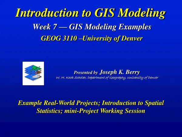
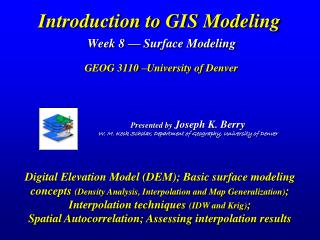
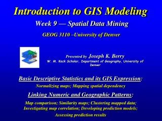
Presented by Joseph K. Berry W. M. Keck Scholar, Department of Geography, University of Denver. Introduction to GIS Modeling Week 9 — Spatial Data Mining GEOG 3110 –University of Denver. Basic Descriptive Statistics and its GIS Expression : Normalizing maps; Mapping spatial dependency

E N D
Presented byJoseph K. Berry W. M. Keck Scholar, Department of Geography, University of Denver Introduction to GIS ModelingWeek 9 — Spatial Data MiningGEOG 3110 –University of Denver Basic Descriptive Statistics and its GIS Expression: Normalizing maps; Mapping spatial dependency Linking Numeric and Geographic Patterns: Map comparison; Similarity maps; Clustering mapped data; Investigating map correlation; Developing prediction models; Assessing prediction results
Kicking for the Finish Exercise #9— to tailor your work to your interests, you can choose to not complete this standard exercise, however in lieu of the exercise you will submit a short paper (4-8 pages) on a GIS modeling topic of your own choosing. Due 5:00 pm Thursday, March 11th. Optional Exercises— you can turn in these exercises for extra credit anytime before 5:00 pm, Tuesday, March 16th. Final Exam Study Questions— covering weeks 7-10, Spatial Statistics and Future Directions; the exam is optional and can only improve your grade. You are encouraged to study together and exchange insights about answering the questions. …at least three-fourths of the exam will be taken directly (verbatim) from the list of study questions. The format will be similar to the last exam, with questions from Terminology, Procedures and Basic Concepts, How Things Work and Mini-Exercises. …study questionsfor Exam 2 are posted on the class website now; send me an email if a question needs further explanation and I will post the clarification. Final Exam— Covers material from weeks 7 (GIS Modeling), 8 (Surface Modeling), 9 (Spatial data Mining) and 10 (Future Directions) …exam posted on the class website by 10:00 am, Thursday, March 11thand must be completed by 5:00 pm, Tuesday, March 16th. … at the end of the last class I will be handing out a CD with all of the class material— sort of a “graduation present” that will keep you GIS-ing for years (Berry)
An Analytic Framework for GIS Modeling (Last week) Surface Modellingoperations involve creating continuous spatial distributions from point sampled data (univariate). (This week) Spatial Data Miningoperations involve characterizing numerical patterns and relationships among mapped data (multivariate). See www.innovativegis.com/basis/Download/IJRSpaper/ (Berry)
Basic Concepts in Statistics (Standard Normal Curve) See Beyond Mapping III , Topic 7, Linking Data Space and Geographic Space (Berry)
Basic Concepts in Statistics (SN_Curve Shape) Kurtosis…shape (positive= peaked; negative= flat) See Beyond Mapping III , Topic 7, Linking Data Space and Geographic Space (Berry)
Basic Concepts in Statistics (SN_Curve Shape continued) …Multi-modal …Skewness (positive= right; negative= left) See Beyond Mapping III , Topic 7, Linking Data Space and Geographic Space (Berry)
Antenna Offset GPS Fix Delay Overlap and Multiple Passes Mass Flow Lag and Mixing Preprocessing Mapped Data (Preprocessing Types 1-3) • Preprocessinginvolves conversion of raw data into consistent units that accurately represent mapped conditions(4 considerations) • Calibration1 — “tweaking” the values… sort of like a slight turn on a bathroom scale to alter the reading to what you know is your ‘true weight’ • Translation2 — converts map values into appropriate units for analysis, such as feet into meters or bushels per acre (measure of volume) into tons per hectare (measure of mass) • Adjustment/Correction3— • dramatically changes the • data, such as post processing • GPS coordinates and/or Mass Flow Lag adjustment (Berry)
Normalizing Mapped Data (4th type of preprocessing) Applying normalization… Norm_GOAL = (Yield_Vol / 250 ) * 100 …generates a standardized map based on a yield goal of 250 bushels/acre. This map can be used in analysis with other goal-normalized maps, even from different crops Since normalization involves scalar mathematics (constants), the pattern of the numeric distribution (histogram) and the spatial distribution (map) do not change …same relative distributions • Normalization4— involves standardization of a data set, usually for comparison among different types of data… • Goal…Norm_GOAL = (mapValue / 250 ) * 100 • 0-100…Norm_0-100 = ((mapValue – min) * 100) / (max – min) • SNV…Norm_SNV = ((mapValue - mean) / stdev) * 100 Key Concept (Berry) See Beyond Mapping III , Topic 18, Understanding Grid-based Data
Assessing Localized Variation Question 1 – Visual Map Analysis (Spatial and Numeric distributions) Scan Yield_Volume Coffvar Within 2 For Yield_Coffvar Where, Coffvar = Stdev/mean *100 The “Scan” operation moves a window around the yield map and calculates the Coefficient of Variation with a 2-cell radius of each location …higher values indicate areas with more localized variability CoffVar= (StDev/Mean) * 100 (Berry)
…unusually high yield …proximity to high yield areas …Yield map > Average + 1Stdev Data Proximity/Buffer Stratification …proximity to field edge …Stratificationpartitions the data (numeric) or the project area (spatial) into logical groups— Edge effects “Sweet Spot” (interior) …Proximity mapidentifies the distance from point, line or polygon features to all other locations Far : Close “High Yield” vicinity (Berry)
…creates a map summarizing values from a data map (Phosphorous levels) that coincide with the categories of a template map (Soil types) BIB Soil Type Ve VdC BIB BIA TuC HvB Pavg 15.0 12.8 11.2 14.6 10.5 11.3 Overall BIA Pavg = 14.6 …average phosphorous level for each soil type 13.6 15.5 8.6 …average P-level for each soil unit (clump first before COMPOSITE) Summarizing Map Regions(template/data) Soil Types Phosphorous levels (Berry)
Comparing Discrete Maps (Multivariate analysis) Thematic Categorization …we often represent continuous spatial data (map surfaces) as a set of discrete polygons Which classified map is correct? How similar are the three maps? Spatial Precision (Where — boundaries) of Points, Lines and Areas (polygons) is a primary concern of GIS, but we are often less concerned with Thematic Accuracy (What — map values) High Medium Low (Berry) See Beyond Mapping III , Topic 10, Analyzing Map Similarity and Zoning
Comparing Discrete Maps Two ways to compare Discrete Maps… Coincidence Summary Proximal Alignment …Coincidence Summary generates a cross-tabular listing of the intersection of two maps. Table Interpretation Diagonal (Same) Off-diagonal (Above/Below) Percentages (% Same) Overall Percentage ((631+297+693)/1950)*100= 83% ((475+297+563)/1950)*100=68% Raster versus Vector 693 See Beyond Mapping III , Topic 10, Analyzing Map Similarity and Zoning (Berry)
Comparing Discrete Maps Two ways to compare Discrete Maps… Coincidence Summary Proximal Alignment Map2: Med-- 104 + 297 + 225 = 626; (297/626) *100= 47 percent matched 631 + 297 + 693 = 1621; (1621/1950) *100= 83 percent matched 475 + 297 + 563 = 1335; (1335/1950) *100= 68 percent matched Map3: Med-- 260 + 297 + 335= 912; (297/912) *100= 36 percent matched Question 2 Map1 …Coincidence Summary generates a cross-tabular listing of the intersection of two maps. Table Interpretation Diagonal (Same) Off-diagonal (Above/Below) Percentages (% Same) Overall Percentage ((631+297+693)/1950)*100= 83% ((475+297+563)/1950)*100=68% Raster versus Vector Map2 Map1 Map3 See Beyond Mapping III , Topic 10, Analyzing Map Similarity and Zoning (Berry)
Diagonal elements in the map comparison matrix identify agreement (matches) between two progressive ordinal maps Low Med High Total 208 0 0 208/208 = 100% Off-diagonal elements in the map comparison matrix identify disagreement (miss-matches) between two progressive ordinal maps Low 0 208 0 208/208 = 100% Med Low Med High Total 0 0 208 208/208 = 100% …ALL MISMATCHES where there is an opposite relationship Overall coincidence = 0% High 69 70 69 69/208 = 33% Low 208/208 = 100% 208/208 = 100% 208/208 = 100% 624/624 = 100% Total 70 69 69 69/208 = 33% Med …PERFECT COINCIDENCE where all of the increasing ordinal steps are matched (diagonal) and there is no mismatches (off-diagonal). Overall coincidence is 624/624 = 100% found by the sum of the diagonal elements (matches); the other totals indicate percent agreement by category on each map Low Med High Total 69 69 70 69/208 = 33% High 0 104 104 0/208 = 0% Low 69/208 = 33% 69/208 = 33% 69/208 = 33% 208/624 = 33% Total 104 0 104 0/208 = 0% Med …EQUALLY BALANCED matches and mismatches where there is no pattern relationship Overall coincidence = 33% partially matched and mismatched 104 104 0 0/208 = 0% High 0/208 = 0% 0/208 = 0% 0/208 = 0% 0/624 = 0% Total Coincidence Table (idealized conditions) (Berry)
Comparing Discrete Maps Two ways to compare Discrete Maps… Coincident Summary Proximal Alignment …Proximal Alignment isolates a category on one of the maps, generates its proximity, then identifies the proximity values that align with the same category on the other map. Table Interpretation Zeros (Agreement) Values (> Disagreement) PA Index (average) Proximity_Map1_Category1 * Binary_Map3_Category1 …non-zero values identify changes and how far away (Berry) See Beyond Mapping III , Topic 10, Analyzing Map Similarity and Zoning
Comparing Map Surfaces (Statistical Tests) Three ways to compare Map Surfaces… Statistical Tests Percent Difference Surface Configuration …Statistical Tests compare one set of cell values to that of another based on the differences in the distributions of the data— 1) data sets (partition or coincidence; continuous or sampled) 2) statistical procedure (t-Test, f-Test, etc.) Box-and-whisker graphs (Berry) See Beyond Mapping III , Topic 10, Analyzing Map Similarity and Zoning
Comparing Map Surfaces (%Difference) Three ways to compare Map Surfaces… Statistical Tests Percent Difference Surface Configuration Question 3 …Percent Difference capitalizes on the spatial arrangement of the values by comparing the values at each map location— %Difference Map, %Difference Table (Berry) See Beyond Mapping III , Topic 10, Analyzing Map Similarity and Zoning
Comparing Map Surfaces (Surface Configuration) Three ways to compare Map Surfaces… Statistical Tests Percent Difference Surface Configuration …Surface Configuration capitalizes on the spatial arrangement of the values by comparing the localized trend in the values — Slope Map, Aspect Map, Surface Configuration Index (Berry) See Beyond Mapping III , Topic 10, Analyzing Map Similarity and Zoning
Comparing Map Surfaces(Temporal Difference) 1997_Yield_Volume - 1998_Yield_Volume Map Variables… map values within an analysis grid can be mathematically and statistically analyzed = Yield_Diff …green indicates areas of increased production …yellow indicates minimal change …red indicates decreased production (Berry) See Beyond Mapping III , Topic 16, Characterizing Patterns and Relationships
Data Analysis(establishing relationships) On-farm studies, such as seed hybrid performance, can be conducted using actual farm conditions… …management action recommendations are based on local relationships instead of Experiment Station research hundreds of miles away …is radically changing research and management practicesin agriculture and numerous other fields from business to epidemiology and natural resources (Berry)
Map Stack– relationships among maps are investigated by aligning grid maps with a common configuration… #cols/rows, cell size and geo-reference. Data Shishkebab– each map represents a variable, each grid space a case and each value a measurement with all of the rights, privileges, and responsibilities of non-spatial mathematical , numerical and statistical analysis Spatial Dependency • Spatial Variable Dependence— what occurs at a location in geographic space is related to: • the conditions of that variable at nearby locations, termed Spatial Autocorrelation (intra-variable dependence) • the conditions of other variables at that location, termed Spatial Correlation (inter-variable dependence) (Berry) See Beyond Mapping III , Topic 16, Characterizing Patterns and Relationships
Interpolated Spatial Distribution Phosphorous (P) What spatial relationships do you see? Visualizing Spatial Relationships …do relatively high levels of P often occur with high levels of K and N? …how often? …where? (Berry) See Beyond Mapping III , Topic 16, Characterizing Patterns and Relationships
Identifying Unusually High Measurements …isolate areas with mean + 1 StDev (tail of normal curve) (Berry) See Beyond Mapping III , Topic 16, Characterizing Patterns and Relationships
Level Slicing …simply multiply the two maps to identify joint coincidence 1*1=1 coincidence (any 0 results in zero) Question 4 (Berry) See Beyond Mapping III , Topic 16, Characterizing Patterns and Relationships
Multivariate Data Space …sum of a binary progression (1, 2 ,4 8, 16, etc.) provides level slice solutions for many map layers (Berry) See Beyond Mapping III , Topic 16, Characterizing Patterns and Relationships
Calculating Data Distance …an n-dimensional plot depicts the multivariate distribution; the distance between points determines the relative similarity in data patterns …the closest floating ball is the least similar (largest data distance) from the comparison point (Berry) See Beyond Mapping III , Topic 16, Characterizing Patterns and Relationships
Identifying Map Similarity Question 5 …the relative data distance between the comparison point’s data pattern and those of all other map locations form a Similarity Index The green tones indicate field locations with fairly similar P, K and N levels; red tones indicate dissimilar areas. (Berry) See Beyond Mapping III , Topic 16, Characterizing Patterns and Relationships
…a map stack is a spatially organized set of numbers Cyber-Farmer, Circa 1992 …groups of “floating balls” in data space identify locations in the field with similar data patterns– data zones …fertilization rates vary for the different clusters “on-the-fly” Variable Rate Application Clustering Maps for Data Zones Question 6 (Berry) See Beyond Mapping III , Topic 16, Characterizing Patterns and Relationships
Assessing Clustering Results …Clustering results can be roughly evaluated using basic statistics Average, Standard Deviation, Minimum and Maximum values within each cluster are calculated. Ideally the averages between the two clusters would be radically different and the standard deviations small—large difference between groups and small differences within groups. Standard Statistical Tests of two data sets Box and Whisker Plots to visualize differences (Berry) See Beyond Mapping III , Topic 16, Characterizing Patterns and Relationships
How Clustering Works (IsoData algorithm) The scatter plot shows Height versus Weight data that might have been collected in your old geometry class The data distance to each weight/height measurement pair is calculated and the point is assigned to the closest arbitrary cluster center Repeat data distances, cluster assignments and repositioning until no change in cluster membership (centers do not move) The average X,Y coordinates of the assigned students is calculated and used to reposition the cluster centers (Berry) See Beyond Mapping III , Topic 7, Linking Data Space and Geographic Space
Spatial Data Mining (The Big Picture) …making sense out of a map stack Mapped data that exhibits high spatial dependency create strong prediction functions. As in traditional statistical analysis, spatial relationships can be used to predict outcomes …the difference is that spatial statistics predicts where responses will be high or low (Berry) See Beyond Mapping III , Topic 16, Characterizing Patterns and Relationships
An Analytic Framework for GIS Modeling This Week Spatial Data Mining operations involve characterizing numerical patterns and relationships among mapped data. See www.innovativegis.com/basis/Download/IJRSpaper/ (Berry)
Regression (conceptual approach) A line is “fitted” in data space that balances the data so the differences from the points to the line (residuals) for all the points are minimized and the sum of the differences is zero… …the equation of the regression line is used to predict the “Dependent” variable (Y axis) using one or more “Independent” variables (X axis) (Berry)
Non-spatial…R-squared value looks at the deviations from the regression line; data patterns about the regression line Evaluating Prediction Maps (non-spatial) (Berry)
The Dependent Map variable is the one that you want to predict… …derive from customer data …from a set of existing or easily measured Independent Map variables Map Variables Question 7 (Berry) See Beyond Mapping III , Topic 28, Spatial Data Mining in Geo-Business
Scatter plots and regression equations relating Loan Density to three candidate driving variables (Housing Density, Value and Age) Loans= fn( Housing Density ) Loans= fn( Home value ) Loans= fn( Home Age ) The “R-squared index” provides a general measure of how good the predictions ought to be— 40%, 46% indicates a moderately weak predictors; 23% indicates a very weak predictor (R-squared index = 100% indicates a perfect predictor; 0% indicates an equation with no predictive capabilities) Map Regression Results (Bivariate) Question 8 (Berry) See Beyond Mapping III , Topic 28, Spatial Data Mining in Geo-Business
Generating a Multivariate Regression …a regression equation using all three independent map variables using multiple linear regression is used to generate a prediction map Question 9 (Berry) See Beyond Mapping III , Topic 28, Spatial Data Mining in Geo-Business
Evaluating Regression Results (multiple linear) Optional Question 9-1 …a regression equation using all three independent map variables using multiple linear regression is used to generate a prediction map …that is compared to the actual dependent variable data — Error Surface (Berry) See Beyond Mapping III , Topic 28, Spatial Data Mining in Geo-Business
Using the Error Map to Stratify One way to improve the predictions, however, is to stratify the data set by breaking it into groups of similar characteristics …and then generating separate regressions …generate a different regression for each of the stratified areas– red, yellow and green …other stratification techniques include indigenous knowledge, level-slicing and clustering (Berry) See Beyond Mapping III , Topic 28, Spatial Data Mining in Geo-Business
An Analytic Framework for GIS Modeling This Week Spatial Data Mining operations involve characterizing numerical patterns and relationships among mapped data. See www.innovativegis.com/basis/Download/IJRSpaper/ (Berry)
Prescriptive Mapping • Four primary types of applied spatial models: • Suitability—mapping preferences (e.g., Habitat and Routing) • Economic— mapping financial interactions (e.g., Combat Zone and Sales Propensity) • Physical—mapping landscape interactions (e.g., Terrain Analysis and Sediment Loading) • Mathematical/Statistical— mapping numerical relationships… • Descriptivemath/stat models summarize existing mapped data • (e.g., Standard Normal Variable Map for Unusual Conditions and Clustering for Data Zones) • Predictivemath/stat models develop equations relating mapped data • (e.g., Map Regression for Equity Loan Prediction and Probability of Product Sales ) • Prescriptivemath/stat models identify management actions based on descriptive/predictive relationships (e.g., Retail Marketing and Precision Ag)… • Discrete Actions: If <condition(s)> Then <Action(s)> • If P is 0-4 ppm, then apply 50 lbs P2O5/Acre • If P is 4-8 ppm, then apply 30 lbs P2O5/Acre • If P is 8-12 ppm, then apply 15 lbs P2O5/Acre • If P is >12 ppm, then apply 0 lbs P2O5/Acre 50 50 30 15 0 0 • Continuous Actions: Equation defining action(s) • Negative linear equation of the form:y = aX • Negative exponential equation of the form: y = e-x 0 P 12 more Phosphorous (P) P2O5/ 50 P2O5/ 0 (Berry) 0 P 12 more
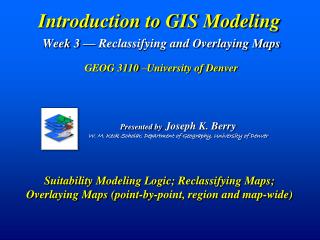
Grid-Based Map Analysis • Spatial analysisinvestigates the “contextual” relationships in mapped data… • Reclassify— reassigning map values (position; value; size, shape; contiguity) • Overlay— map overlay (point-by-point; region-wide) • Distance— proximity and connectivity (movement; optimal paths; visibility) • Neighbors— ”roving windows” (slope/aspect; diversity; anomaly) ...Whew!!! • Surface modelingmaps the spatial distribution and pattern of point data… • Density Analysis— count/sum of points within a local window • Spatial Interpolation— weighted average of points within a local window • Map Generalization— fits mathematical relationship to all of the point data • Spatial data mininginvestigates the “numerical” relationships in mapped data… • Descriptive— summary statistics, comparison, classification (e.g., clustering) • Predictive— math/stat relationships among map layers (e.g., regression) • Prescriptive— appropriate actions (e.g., optimization) (Berry)
Kicking for the Finish Exercise #9— to tailor your work to your interests, you can choose to not complete this standard exercise, however in lieu of the exercise you will submit a short paper (4-8 pages) on a GIS modeling topic of your own choosing. Due 5:00 pm Thursday, March 11th. Optional Exercises— you can turn in these exercises for extra credit anytime before 5:00 pm, Tuesday, March 16th. Final Exam Study Questions— covering weeks 7-10, Spatial Statistics and Future Directions; the exam is optional and can only improve your grade. You are encouraged to study together and exchange insights about answering the questions. …at least three-fourths of the exam will be taken directly (verbatim) from the list of study questions. The format will be similar to the last exam, with questions from Terminology, Procedures and Basic Concepts, How Things Work and Mini-Exercises. …study questionsfor Exam 2 are posted on the class website now; send me an email if a question needs further explanation and I will post the clarification. Final Exam— Covers material from weeks 7 (GIS Modeling), 8 (Surface Modeling), 9 (Spatial data Mining) and 10 (Future Directions) …exam posted on the class website by 10:00 am, Thursday, March 11thand must be completed by 5:00 pm, Tuesday, March 16th. … at the end of the last class I will be handing out a CD with all of the class material— sort of a “graduation present” that will keep you GIS-ing for years (Berry)