Spatial Data Mining
Spatial Data Mining. Introduction. Spatial data mining is the process of discovering interesting, useful, non-trivial patterns from large spatial datasets E.g. co-location patterns of water pumps and cholera Determining hotspots: unusual locations Spatial Data Mining Tasks

Spatial Data Mining
E N D
Presentation Transcript
Introduction • Spatial data mining is the process of discovering interesting, useful, non-trivial patterns from large spatial datasets • E.g. co-location patterns of water pumps and cholera • Determining hotspots: unusual locations • Spatial Data Mining Tasks • Classification/Prediction • Co-location Mining • Clustering • Recap of special properties of Spatial Data • Spatial autocorrelation • Spatial heterogeneity • Implicit Spatial Relations
Spatial Relations • Spatial databases do not store spatial relations explicitly • Additional functionality required to compute them • Three types of spatial relations specified by the OGC reference model • Distance relations • Euclidean distance between two spatial features • Direction relations • Ordering of spatial features in space • Topological relations • Characterise the type of intersection between spatial features
If dist is a distance function and c is some real number dist(A,B)>c, dist(A,B)<c and dist(A,B)=c Distance relations A B A B A B
If directions of B and C are required with respect to A Define a representative point, rep(A) rep(A) defines the origin of a virtual coordinate system The quadrants and half planes define the direction relations B can have two values {northeast, east} Exact direction relation is northeast Direction relations C north A C B northeast A B A rep(A)
Topological Relations • Topological relations describe how geometries intersect spatially • Simple geometry types • Point, 0-dimension • Line, 1-dimension • Polygon, 2-dimension • Each geometry represented in terms of • boundary (B) – geometry of the lower dimension • interior (I) – points of the geometry when boundary is removed • exterior (E) – points not in the interior or boundary • Examples for simple geometries • For a point, I = {point}, B={} and E={Points not in I and B} • For a line, I={points except boundary points}, B={two end points} and E={Points not in I and B} • For a polygon, I={points within the boundary}, B={the boundary} and E={points not in I and B}
DE-9IM • Topological relations are defined using any one of the following models • 4IM, four intersection model (only B and E considered) • 9IM, nine intersection models (B, I, and E) • DE-9IM, dimensionally extended 9 intersection model • DE-9IM is an OGC complaint model • Dim is the dimension function
Consider two polygons A - POLYGON ((10 10, 15 0, 25 0, 30 10, 25 20, 15 20, 10 10)) B - POLYGON ((20 10, 30 0, 40 10, 30 20, 20 10)) Example
E(B) I(B) B(B) I(A) B(A) E(A) 9-Intersection Matrix of example geometries
Relationships using DE-9IM • Different geometries may give rise to different numbers in the DE-9IM • For a specific type of relationship we are only interested in certain values in certain positions • That is, we are interested in patterns in the matrix than actual values • Actual values are replaced by wild cards • T: value is "true" - non empty - any dimension >= 0 • F: value is "false" - empty - dimension < 0 • *: Don't care what the value is • 0: value is exactly zero • 1: value is exactly one • 2: value is exactly two
Topological Relations • x.Disjoint(y) • FF*FF**** • x.Touches(y) • FT******* Area/Area, Line/Line, Line/Area, Point/Area • F**T***** Not Point/Point • F***T**** • x.Crosses(y) • T*T****** Point/Line, Point/Area, Line/Area • 0******** Line/Line • x.Within(y) • TF*F***** • x.Overlaps(y) • T*T***T** Point/Point, Area/Area • 1*T***T** Line/Line • DE-9IM string for example geometries was ‘212101212’ (from earlier slide) • A crosses B • A overlaps B
Approaches to Spatial Data Mining • Materialize spatial features and use Weka • Required features are added as additional attributes to the main feature • To create a flat file of data • Use special data mining techniques that take spatial dependency into account
Retrieve data belonging to multiple themes Preprocess spatial data to materialize spatial features Select the required features Use the methods to compute spatial relations to create a flat file of data Use Weka like tool to perform data mining Spatial Data Mining Architecture Weka Flat File Feature Selection & OGC complaint methods to compute relations Multiple Themes OGC Complaint Spatial DBMS
Spatial Clustering • Also called spatial segmentation • Input • a table of area names and their corresponding attributes such as population density, number of adult illiterates etc. • Information about the neighbourhood relationships among the areas • A list of categories/classes of the attributes • Output • Grouped (segmented) areas where each group has areas with similar attribute values • Census Website has plenty of examples • http://www.statistics.gov.uk/census2001/censusmaps/index.html
Similarity with image segmentation • Spatial segmentation is performed in image processing • Identify regions (areas) of an image that have similar colour (or other image attributes). • Many image segmentation techniques are available • E.g. region-growing technique
There are many flavours of this technique One of them is described below: Assign seed areas to each of the segments (classes of the attribute) Add neighbouring areas to these segments if the incoming areas have similar values of attributes Repeat the above step until all the regions are allocated to one of the segments Functionality to compute spatial relations (neighbours) assumed Region Growing Technique 1 1 1 1 1 1 2 2 2 2 2 2 2
Summary • Spatial data storage available as extensions of RDBMS • Visualization of Spatial data available in GIS • Spatial Data Mining requires functionality to compute spatial relations • OGC specifications provide the standards for all the above resources • MYSQL provides data spatial data storage • But only partially provides the functionality for computing relations • Several OpenSource systems provide all the above resources for spatial data • OpenJump, GeoTools