Download
1 / 42
480 likes | 736 Views
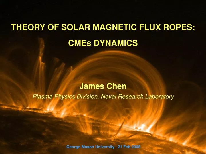
THEORY OF SOLAR MAGNETIC FLUX ROPES: CMEs DYNAMICS. James Chen Plasma Physics Division, Naval Research Laboratory. George Mason University 21 Feb 2008. Canonical parameters of solar eruptions: KE, photons, particles erg Mass g Speed ~100 - 2000 km/s

E N D
THEORY OF SOLAR MAGNETIC FLUX ROPES:CMEs DYNAMICS James Chen Plasma Physics Division, Naval Research Laboratory George Mason University 21 Feb 2008
Canonical parameters of solar eruptions: • KE, photons, particles erg • Mass g • Speed ~100 - 2000 km/s • Space Weather: CMEs are the solar drivers of large geomagnetic storms • Physical mechanism: CMEs lead to strong-B solar wind (SW) structures (i.e., strong southward IMF) impinging on the magnetosphere • CMEs are magnetically dominated structures SOLAR ERUPTIONS
SOHO new capabilities and insight SCIENTIFIC CHALLENGES Observational challenges: • All remote sensing • Different techniques observe different aspects/parts of an erupting structure (Twenty blind men …) • 3-D geometry not directly observed Theoretical challenges: • A major unsolved question of theoretical physics • Energy source – poorly understood • Underlying B structure – not established • Driving force (“magnetic forces”) uncertain
A FLUX-ROPE CME LASCO C2 data: 12 Sept 2000 CME leading edge (ZLE) x EP (Zp) Chen (JGR, 1996)
OBSERVATIONAL EVIDENCE (No prominence included) • Good quantitative agreement with a flux rope viewed end-on(Chen et al. 1997) • No evidence of reconnection • Other examples of flux-rope CMEs(Wood et al. 1999; Dere et al., 1999; Wu et al. 1999; Plunkett et al. 2000; Yurchyshyn 2000; Chen et al. 2000; Krall et al. 2001)
OBSERVATIONAL EVIDENCE (cont’d) • A flux-rope viewed from the side • Halo CMEs are flux ropes viewed head on [Krall et al. 2005] (No prominence included)
3-D GEOMETRY OF CMEs • “Coronal transients”(1970’s: OSO-7, Skylab) • “Thin” flux tubes (Mouschovias and Poland 1978; Anzer 1978) • Halo CMEs (Solwind) (Howard et al. 1982) • Fully 3-D in extent • CME morphology (SMM): (Illing and Hundhausen 1986) • A CME consists of 3-parts: a bright frontal rim, cavity, and a core • Conceptual structure: rotational symmetry (e.g., ice cream cone, light bulb) (Hundhausen 1999) • SOHO data: 3-D flux ropes (Chen et al. 1997) • 3-part morphology is only part of a CME FOV: 1.7 – 6 Rs (Illing and Hundhausen (1986) SMM(1980-1981; 1984-1989)
CME GEOMETRY WITH ROTATIONAL SYMMETRY • Rotationally symmetric model (e.g., Hundhausen1999) and some recent models (SMM) (1970s vintage) No consistent magnetic field
THEORETICAL CONCEPTS: TWO MODEL GEOMETRIES Magnetic Arcades (Traditional flare model) Magnetic Flux Ropes Magnetic arcade-to-flux rope • Energy release and formation of flux rope during eruption (e.g., Antiochos et al. 1999; Chen and Shibata 2000; Linker et al. 2001) Poynting flux S = 0 through the surface Not yet quantitative agreement with CMEs Pre-eruption structure: flux rope with fixed footpoints (Sf) (Chen 1989; Wu et al. 1997; Gibson and Low 1998; Roussev et al. 2003) through the surface (Chen 1989)
pa GENERAL 1D FLUX ROPE • Consider a 1-D straight flux rope • Embedded in a background plasma of pressure pa • MHD equilibrium: • r = a : minor radius • Momentum equation: • Requirements for B: • Toroidal (locally axial) field: Bt(r) Poloidal (locally azimuthal) field: Bp(r)
1D FLUX ROPE EQUILIBRIA • Problem to solve: specify the system environment pa and find a solution • General solution: • For any given pa, there is an inifinity of solutions • Must satisfy • Problem: What is the general form of B(x) in 1D?
1D FLUX ROPE EQUILIBRIA • Two-parameter family of solutions; where • Equilibrium limit: p(0) > 0
A SPECIFIC EQUILIBRIUM SOLUTION • Constraints: Seek simplest solutions with one scale length (a): use the smallest number of terms in r/a satisfying div B = 0. Demand that there be no singularities and that current densities vanish continuously at r = a. • Problem: (1) Show that the following field satisfies div B = 0. (2) Then find p(r), Jp(r), and Jt(r) for equilibrium. Note that Jp(r) must vanish at r = 0 (to avoid a singularity) and r = a. Therefore, Jp(r) must have its maximum near r/a = ½.
EQUILIBRIUM BOUNDARY • Problem: (1) Derive the equilibrium condition for given pa. Show that the equilibrium boundary asymptotes to the straight line (2) What is the physical meaning of the asymptote?
A SPECIFIC EQUILIBRIUM SOLUTION • Problem: (1) Find representative solutions to verify the general characteristics. Plot the the results for different regimes. (2) Calculate the local Alfven speed inside and outside the current channel based on the total magnetic field. Express the results in terms of the ion thermal speed, assuming constant temperature. (3) Show boundary curve on the plot
GOLD-HOYLE FLUX ROPE • Repeat the same exercises using the Gold-Hoyle flux rope. That is, find p(r), Jp(r), and Jt(r). • Describe the physical meaning of the parameter q? Define . Derive a constraint on in terms of q.
pa TOROIDICITY • Symmetric straight cylinder in a uniform background pressure: • All forces are in theminor radial direction • Toroidicity in and of itself introducesmajor radialforces
TOROIDICITY • Consider a toroidal current channel embedded in a background plasma of uniform pressure pa • Average internal pressure: • Toroidicity in and of itself introducesmajor radialforces • Problem: Show pa
R LORENTZ (HOOP) FORCE • Self-force in the presence of major radial curvature; Biot-Savart law • Consider an axisymmetric toroidal current-carrying plasma Shafranov (1966, p. 117); Landau and Lifshitz (1984, p. 124); Garren and Chen (Phys. Plasmas1, 3425, 1994); Miyamoto (Plasma Physics for Nuclear Fusion, 1989)
R LORENTZ (HOOP) FORCE • Perturb UT about equilibrium (F = 0) • Assume idel MHD and adiabatic for the perturbations • Total force acting on the torus: • Major radial force per unit length: • Minor radial force per unit length:
APPLICATION TO SOLAR FLUX ROPES • Solar flux ropes: • Non-axisymmetric • R/a is not uniform • Eruptive phenomena: • Shafranov’s derivation is for equilibrium (FR = 0 and Fa= 0) • CMEs are highly dynamic • Drag and gravity • Application to CMEs: Assumptions
SOLAR FLUX ROPES: NON-AXISYMMETRIC GEOMETRY • Non-axisymmetric • Assume one average major radius of curvature during expansion, R • Stationary footpoints with separation Sf • Height of apex, Z • However, the minor raidus cannot be assumed to be uniform
SOLAR FLUX ROPES: INDUCTANCE • Inducatance L: Definition • Problem:: Show specific forms for the following choice of • Minor radius exponentially increases from footpoints to apex • Linearly increases from footpoints
SOLAR FLUX ROPES: INDUCTANCE • Generally, as a flux rope expands, • Problem: Assume that Show that as a flux rope expands, its magnetic energy decreases as
SOLAR FLUX ROPES: INTERACTION WITH CORONA • Dynamically, the most important interaction is momentum coupling (i.e., forces) • Drag: Flow around flux rope is not laminar (high magnetic Reynolds’ number) • Gravity:
EQUATIONS OF MOTION Major Radial Equation of Motion: (For simplicity, set Bct = 0) • Original derivation: Shafranov (1966) for axisymmetric equilibrium • Adapted for dynamics of non-axisymmetric solar flux ropes (Chen 1989)
Fa EQUATIONS OF MOTION Major Radial Equation of Motion: (For simplicity, set Bct = 0) • Original derivation: Shafranov (1966) for axisymmetric equilibrium • Adapted for dynamics of non-axisymmetric solar flux ropes (Chen 1989) Minor Radial Equation of Motion:
Fits morphology and dynamics Fits non-trivial speed / acceleration profiles 11 events published [Krall et al., 2001 (ApJ)] COMPARISON WITH LASCO DATA Chen et al. (2000, ApJ)
CHARACTERISTICS OF FLUX-ROPE DYNAMICS Major Radial Equation of Motion:
CHARACTERISTICS OF FLUX-ROPE DYNAMICS Major Radial Equation of Motion:
C2 C2 C2 MAIN ACCELERATION PHASE OF CMEs • CME acceleration profiles • Two phases of acceleration: the main and residual acceleration phases • The main phase: Lorentz force (J x B) dominates • The residual phase: All forces are comparable, all decreasing with height • A general property: verified in ~30 CME and EP events (also Zhang et al. 2001) Calculated forces
PHYSICS OF THE MAIN ACCELERATION PHASE • Basic length scale of the equation of motion • Two critical heights:Z*andZm • Z*: Curvature is maximum (i.e., R is minimum) at apex height Z* (analytic result from geometry) • kR(R) is maximum at • Depends only on the 3-D toroidal geometry with fixed
CHARACTERISTIC HEIGHTS • Zm: For Z > Z*, R monotonically increases • The actual height Zmax of maximum acceleration
EXAMPLES OF OBSERVED CME EVENTS • Example • “CME acceleration is almost instantaneous.” • Bulk of CME acceleration occurs below ~2 — 3 Rs (MacQueen and Fisher 1983; St. Cyr et al. 1999; Vrsnak 2001) • One mechanism is sufficient to account for the “two-classes” of CMEs [Chen and Krall 2003] • Small Sf “Impulsive” • Large Sf “Gradual” (residual phase)
HEIGHT SCALES OF MAIN PHASE: Observation • Test the theory against 1998 June 2 CME: is required
MORE SYSTEMATIC THEORY-DATA COMPARISONS • The Sf -scaling is in good agreement. However, the footpoint separation Sf is not directly measured Use eruptive prominences (EPs) for better Sf estimation Sf = 1.16 RS Zmax = 0.6 RS
DATA ANALYSIS: DETERMINATION OF LENGTHS Reverse video Nobeyama Radioheliograph data Sf = 0.84 RS Zmax = 0.55 RS C2 data
GEOMETRICAL ASSUMPTIONS • The scaling law: most directly given in quantities of flux rope (Z, Sf, Zmax, Z*) • Relationship between CME, prominence, and flux rope quantities • CME leading edge (LE): ZLE = Z + 2aa • Prominence LE: Z = Zp – a • Prominence footpoints: Sp = Sf – 2af • Observed quantities: • Sp, Zp, Zpmax • Calculate: • Sf (Sp, af) • Zmax (Zpmax, aa )
EP data CME data COMPARISON WITH DATA • CMEs: Use magnetic neutral line or H filament to estimate Sf; ZLE = Z + 2a EPs: Sf = Sp + 2af Zp = Z – a 4 CMEs (LASCO) 13 EPs (radio, H ) • A quantitative test of the • accelerating force and • the geometrical assumptions • A quantitative challenge to • all CME models Chen et al., ApJ (2006)
MORE PROPERTIES OF EQUATIONS OF MOTION • Show that during expansion the poloidal field (JtBp) loses energy to the kinetic energy of the flux rope and toroidal field. • Some CME models invoke buoyancy as the driving force. Assuming Fg is the driving force, calculate the terminal speed of the expanding flux rope if the drag is force is taken into account. How fast can buoyancy alone drive a flux rope? • Consider the momentum equation. Assuming that only JxB and pressure gradient force are present, what is the characteristic speed of a magnetized plasma structure of relevant dimension D? What is the characteristic time? • Normalize the MHD momentum equation to the characteristic speed and time for plasma motions in the photosphere and the corona. Can the equations of motion distinguish between the two disparate mediums?