Overview

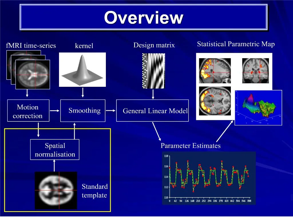
1. Overview

3. Co-registration Term co-registration applies to any method for aligning images By this token, motion correction is also co-registration However, term is usually used to refer to alignment of images from different modalities. E.g.: Low resolution T2* fMRI scan (EPI image) to high resolution, T1, structural image from the same individual

4. Co-registration: Principles behind this step of processing When several images of the same participants have been acquired, it is useful to have them all in register Image registration involves estimating a set of parameters describing a spatial transformation that ‘best ‘ matches the images together

5. fMRI to structural Matching the functional image to the structural image Overlaying activation on individual anatomy Better spatial image for normalisation Two significant differences between co-registering to structural scans and motion correction When co-registering to structural, the images do not have the same signal intensity in the same areas; they cannot be subtracted They may not be the same shape

6. Problem: Images are different Differences in signal intensity between the images

7. Segmentation Use the gray/white estimates from the normalisation step as starting estimates of the probability of each voxel being grey or white matter Estimate the mean and variance of the gray/white matter signal intensities Reassign probabilities for voxels on basis of Probability map from template Signal intensity and distributions of intensity for gray/white matter Iterate until there is a good fit

9. Register segmented images Grey/white/CSF probability images for EPI (T2*) and T1 Combined least squares match (simultaneously) of gray/white/CSF images of EPI (T2*) + T1 segmented images

10. An alternative technique that relies on mutual information theory Different material will have different intensities within a scan modality E.g. air will have a consistent brightness, and this will differ from other materials (such as white matter)

12. SPM co-registration - problems Poor affine normalisation ? bad segmentation etc. Image not homogeneous ? errors in clustering Susceptibility holes in image (e.g. sinuses) ? errors in clustering/segmentation

13. The EPI scans can also be registered to subject’s own mean EPI image Two images from the same subject acquired using the same modality generally look similar Hence, it is sufficient to find the rigid-body transformation parameters that minimise the sum of squared differences between them Easier than co-registration between modalities (intensity correspondence) Can be spatially less precise But more sensitive to detecting activity differences?

15. Normalisation This enables: Signal averaging across participants: Derive group statistics -> generalise findings to population Identify commonalities and differences between groups (e.g., patient vs. healthy) Report results in standard co-ordinate system (e.g. Talairach and Tournoux stereotactic space)

17. Normalisation: Methods Methods of registering images: Label-based approaches: Label homologous features in source and reference images (points, lines, surfaces) and then warp (spatially transform) the images to align the landmarks (BUT: often features identified manually [time consuming and subjective!] and few identifiable landmarks) Intensity-based approaches: Identify a spatial transformation that maximises some voxel-wise similarity measure (usually by minimising the sum of squared differences between images; BUT: assumes correspondence in image intensity [i.e., within-modality consistency], and susceptible to poor starting estimates) Hybrid approaches – combine intensity method with user-defined features

18. SPM: Spatial Normalisation SPM adopts a two-stage procedure to determine a transformation that minimises the sum of squared differences between images: Step 1: Linear transformation (12-parameter affine) Step 2: Non-linear transformation (warping) High-dimensionality problem The affine and warping transformations are constrained within an empirical Bayesian framework (i.e., using prior knowledge of the variability of head shape and size): “maximum a posteriori” (MAP) estimates of the registration parameters

19. Step 1: Affine Transformation Determines the optimum 12-parameter affine transformation to match the size and position of the images 12 parameters = 3 translations and 3 rotations (rigid-body) + 3 shears and 3 zooms

20. Step 2: Non-linear Registration Assumes prior approximate registration with 12-parameter affine step Modelled by linear combinations of smooth discrete cosine basis functions (3D) Choice of basis functions depend on distribution of warps likely to be required For speed and simplicity, uses a “small” number of parameters (~1000)

22. 2-D visualisation (horizontal and vertical deformations): Brain visualisation:

23. Bayesian Framework

24. Algorithm simultaneously minimises: Sum of squared difference between template and source image (update weighting for each base) Squared distance between the parameters and prior expectation (i.e., deviation of the transform from its expected value) Bayesian constraints applied to both: 1) affine transformations based on empirical prior ranges 2) nonlinear deformations based on smoothness constraint (minimising membrane energy) Bayesian Constraints

25. Bayesian Constraints

26. Normalisation: Caveats Constrained to correct for only gross differences; residual variability is accommodated by subsequent spatial smoothing before analysis Structural alignment doesn’t imply functional alignment Differences in gyral anatomy and physiology between participants leads to non-perfect fit. Strict mapping to template may create non-existent features Brain pathology may disrupt the normalisation procedure because matching susceptible to deviations from template image (-> can use brain masks for lesions, etc.; weight different regions differently so they have varied influence on the final solution) Affine transforms not sufficient: Non-linear solutions are required Optimally, move each voxel around until it fits. Millions of dimensions. Trade off dimensionality against performance (potentially enormous number of parameters needed to describe the non-linear transformations that warp two images together; but much of the spatial variability can be captured with just a few parameters) Regularization: use prior information (Bayesian scheme) about what fit is most likely (unlike rigid-body transformations where constraints are explicit, when using many parameters, regularization is necessary to ensure voxels remain close to their neighbours)

27. Normalisation: Solutions Inspect images for distortions before transforming Adjust image position before normalisation to reduce risk of local minima (i.e., best starting estimate) Intensity differences: Consider matching to a local template Image abnormalities: Cost-function masking

28. Sources: Ashburner and Friston’s “Spatial Normalization Using Basis Functions” (Chapter 3, Human Brain Function, 2nd ed.; http://www.fil.ion.ucl.ac.uk/spm/doc/books/hbf2/) Rik Henson’s Preprocessing Slides: http://www.mrc-cbu.cam.ac.uk/Imaging/Common/rikSPM-preproc.ppt Matthew Brett’s Spatial Processing Slides: http://www.mrc-cbu.cam.ac.uk/Imaging/Common/Orsay/jb_spatial.pdf