Download
1 / 19
190 likes | 263 Views
This comprehensive guide delves into long-run and short-run total output, production with fixed and variable inputs, profit maximization, cost behavior, technology factors, market power, and general equilibrium theory in economics. Learn how firms optimize input usage, minimize costs, and achieve production efficiency through practical examples and economic principles.

E N D
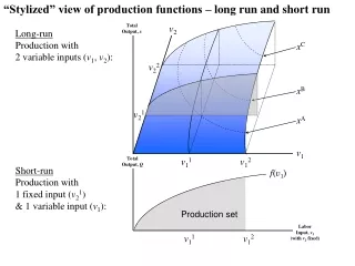
“Stylized” view of production functions – long run and short run Total Output, Q Short-run Production with 1 fixed input (v21) & 1 variable input (v1): Labor Input, v1 (with v2 fixed) Total Output, x v2 Long-run Production with 2 variable inputs (v1, v2): xC v22 xB v21 xA v1 v11 v12 f(v1) Production set v11 v12
Profit Maximization x1 Isoprofit lines with slope x1=f(v1, v2) x1* v1 v1*
Factors Affecting a Firm’s Cost Behavior Technology Factor Costs q q Purchasing Power Market Power of suppliers q q q Diminishing Returns Economies of Scale Economies of Scope The Production Function: x = f(v1, v2) Cost Function Varian, 19.12 (p. 360): If a firm is maximizing profits and if it chooses to supply some output y, then it must be minimizing the cost of producing y. If this were not so, then there would be some cheaper way of producing y units of output, which would mean that the firm was not maximizing profits in the first place. This simple observation turns out to be quite useful in examining firm behavior. It turns out to be convenient to break the profit-maximization problem into two states: first we figure out how to minimize the costs of producing any desired level of output y, then we figure out which level of output is indeed a profit-maximizing level of output…
Long-run production, factor intensity, and optimal input usage Isoquants x2 Total Output, x x1 v2 v2 x0 x2 x1 x0 v1 v1 A “general rule” for efficient input usage:
Long-run production, factor intensity, and factor substitution v2 Elasticity of (factor) substitution: x2 x1 x0 v1
Cost Minimization v2 Isocost lines with slope – w1/w2 v2* Isoquant associated with chosen output v1 v1*
General Equilibrium Theory A General Economy • m consumers • n producers (n goods) • Resources • mX n demand equations • n supply equations Prices A Pure Exchange Economy An economy in which there is no production. A special case of a general economy in which economic activities consist only of trading and consuming. The simplest form of a pure exchange economy is the two-agent, two-good exchange economy, which may be illustrated graphically using the Edgeworth – Bowley Box.
The “Edgeworth Box”: a pure exchange economy B w · x · w · A
The Algebra of Equilibrium Assumptions: Pure exchange economy Two goods: and Two agents, A and B, with … Identical preferences: Arbitrarily determined, but different, endowments: Equilibrium is defined as a consumption bundle Where aggregate excess demands are zero in both markets: Hence, we are seeking a set of prices, , that satisfies these equilibrium conditions.
Pure Exchange and Redistribution – Example from class B · w · w’ · x x’ · A
General Equilibrium Theory A General Economy • m consumers • n producers (n goods) • Resources • mX n demand equations • n supply equations Prices A Production and Exchange Economy A Pure Exchange Economy An economy in which there is no production. A special case of a general economy in which economic activities consist only of trading and consuming. The simplest form of a pure exchange economy is the two-agent, two-good exchange economy, which may be illustrated graphically using the Edgeworth – Bowley Box. To achieve a general equilibrium, an production and exchange economy must simultaneously achieve efficiency in production and efficiency in exchange. = and MRTSi,j1 = MRTSi,j2
Production x2 x2 x2 300 200 100 -2 -1/2 x1 x1 x1 300 100 200 x2 x1 = f(v1, v2) = f(v1) = 10v11 x1 = f(v1, v2) = f(v1) = 20v11 Add a 3rd producer … x2 = g(v1, v2) = g(v1) = 20v12 x2 = g(v1, v2) = g(v1) = 10v12 Resource Constraint: v1 = 10 (Hence, v11 + v12 = 10) Resource Constraint: v1 = 10 (Hence, v11 + v12 = 10) x1/10 + x2/20= 10 x2 = 200 - 2x1 x1/20 + x2/10= 10 x2 = 100 - 1/2x1 x1
The Edgeworth Box used to illustrate a production economy [ ] [ ] Two goods, , produced with two inputs . Allocation of inputs to production: the amount of allocated to production of . -MRTS Red: Isoquants for production of Blue: Isoquants for production of
General Equilibrium: exchange and production [ ] [ ] [ ] Two consumers, , two goods, , produced with two inputs .
Computable General Equilibrium (CGE) Models Production Exchange • Producing Sectors: • Manufacturing • Mineral Extraction • Chemicals and Plastics • Agriculture • Transportation • Public Utilities • Communication • Services • Government • Goods and Services: • Food • Apparel • Consumer Transport • Consumer Services • Business Services • Energy • Housing Output Prices Input Prices
Social Welfare Functions and Social Choice Theory Isowelfare Lines • The “Utilities Possibilities Set” • Any Pareto efficient allocation can be a welfare maximum for some welfare function. • Types of social welfare functions: • - Classical utilitarian • - Rawlsian l Utility Possibility Set • Is it possible to aggregate individual preferences into a coherent social welfare function?
Social Choice Theory: Voting and Aggregation of Preferences Poor Middle Rich A 10% 26% 30% B 15% 24% 36% C 25% 25% 25% Preferences Poor: Middle: Rich: A B C B C A C A B
Social Choice Theory: Arrow’s General Possibility Theorem Kenneth Arrow, Social Choice and Individual Values (1951) Condition 1: Given a set of consistent and transitive individual preferences, a social welfare function should exhibit similar rationality. [Unrestricted scope.] Condition 2: If each individual prefers x to y, then the social welfare function should rank x ahead of y. [Positive association of individual and social values.] Condition 3: The social welfare function’s ordering of x and y should not be altered by the introduction of a third option, z. [Independence of irrelevant alternatives.] Condition 4: The social welfare function is not imposed on society. [Citizens’ sovereignty.] Condition 5: The social welfare function is not a dictatorship. General Possibility Theorem: Given at least three alternative which the members of a society are free to order in any way, every social welfare function that satisfies conditions 1 through 3 is either imposed or dictatorial. F It is impossible to construct an acceptable social welfare function out of individual preference functions.
The “General Theory of the Second Best” R.G. Lipsey and Kelvin Lancaster, “The General Theory of Second Best”, The Review of Economic Studies (1956). Quantity of y Maximization of the objective function U, subject to the blue constraint (a production possibilities frontier) would result in selection of point B, which is technically efficient. Imposition of the second constraint (red) would lead to selection of point A which is preferable to point C even though point C is technically efficient while point A is technically inefficient. l C B l A l Quantity of x The General Theory of the Second Best: If certain constraints within an economic system prevent some efficiency conditions from holding, then, given these secondary constraints, it generally will not be desirable to have the optimum conditions hold elsewhere in the system.