Download
1 / 7
70 likes | 102 Views
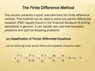
The paper describes the theory of fractional derivative and specific application examples in the field of engineering<br>sciences. On this basis, this paper mainly studies the low reaction-diffusion equations. First using compact operator,<br>the paper constructs a higher-order finite difference scheme. Then the paper proves the existence and uniqueness of<br>the difference solution by matrix method and analyzes the stability and convergence of the scheme by Fourier<br>method.

E N D
Available online www.jocpr.com Journal of Chemical and Pharmaceutical Research, 2014, 6(3):27-33 ISSN : 0975-7384 CODEN(USA) : JCPRC5 ResearchArticle Research and application of compact finite difference method of low reaction-diffusion equation Huancheng Zhang1, Guanchen Zhou1, Yingna Zhao2and Junpeng Yu1 1Qinggong College, Hebei United University, Tangshan, China 2Hebei United University, Tangshan, China _____________________________________________________________________________________________ ABSTRACT The paper describes the theory of fractional derivative and specific application examples in the field of engineering sciences. On this basis, this paper mainly studies the low reaction-diffusion equations. First using compact operator, the paper constructs a higher-order finite difference scheme. Then the paper proves the existence and uniqueness of the difference solution by matrix method and analyzes the stability and convergence of the scheme by Fourier method. Key words: Fractional Differential Equations, Low reaction-diffusion equations, Compact finite difference method, Fourier method _____________________________________________________________________________________________ INTRODUCTION Application of fractional differential equations in the field of engineering sciences is gradually expanded. Especially in recent years, application of fractional differential equations in the field of hydromechanics, viscoelasticity, rheology, fractional control systems and fractional controller, electroanalytical chemistry, electronic circuit and electrically conductive in biological system are more and more [1-3]. There are three fractional derivative definitions: Griinwald-letnikov (G-L) Definition[1], Riemann-Liouville (R-L) Definition[1] and Caputo Definition[2]. R-L Definition: ) 1 d f ( ) t a 1 t d D f ( t ) 1 , 0 ( ), a , b R , a t b , ) ( t f a 1 ( ) dt ( t [ b a , ] Let is continuous on , the R-L fractional differential is ) ( where is Gamma function. 1 t t D f ( t ) f ( ( ) s t s ) ds 0 , t 0 , T . 1 a 1 ( ) a Caputo Definition: Whennegative real number or positive integer, three definitions is can be converted to each other. G-L definition is generally used for discrete computing. R-L and Caputo definition are commonly used in the discussion of fractional differential equations. APPLICATION EXAMPLE (1) Promotion and application of Newton's law f ( a ) ( a ) a ma f mx ( x D 1 , x a ) 2 Wasteland et al [5, 6] propose to Newton's second law of instead of with . 27
Huancheng Zhang et al ______________________________________________________________________________ J. Chem. Pharm. Res., 2014, 6(3):27-33 (2) Conduction applications in biology X ( ) X 0 ( , ) 1 In the study of biological electrical conduction, experts give the transfer function where is current frequency, 0 X and 0 are constant and their values are ) ( s G S associated with the cell type. G If we see the above formula as Laplace transform, i.e. g Dl , then L inverse transformation is fractional 0 ( t ) 0 , 0 1 differential equation . 0 D PI (3)Application of controller U ( s ) G ( s ) k k s k s , , 0 k , k , k p I D D E ( s ) PI p l The function of controller is ) ( t e D where constants are and D k k D e ( t ) k e ( t ) u ( t ) the output equation is . l D p 1 , 1 0 For the above formula, if , then it is the traditional PID controller; if , then it is PI , 0 1 0 controller; if , then it is PD controller; if , we give a gain. (4)Application of Fractional control system D PI The system equation of controller is n t a D y ( t ) k y k D y ( t ) k D y ( t ) k w ( t ) k D w ( t ) k D w ( t ) k k p I D p I D k 0 k s k k s p I D closed G ( s ) m k a s k s k k s k k p I D 0 Where the transfer function is . n a D y ( t ) k w ( t ) k D w ( t ) k D w ( t ) k k p I D If the system is open-loop system, then the differential equation is . k 0 COMPACT FINITE DIFFERENCE METHOD OF LOW REACTION-DIFFUSION EQUATION Derivation of the equation General reaction-diffusion equation set is the following: 2 a ( x , t ) D a ( x , t ) a ( x , t ) b ( x , t ) 2 t x (1) 2 b ( x , t ) D b ( x , t ) a ( x , t ) b ( x , t ) 2 t x (2) Where D is diffusion constant. When the particle movement and reactions are affected by the low diffusion factor, equation set can be developed in the following form 2 1 t a ( x , t ) D a ( x , t ) a ( x , t ) b ( x , t ) 0 2 t x (3) 2 2 1 t b ( x , t ) D b x , t a ( x , t ) b ( x , t ) 0 2 t x (4) Dt 1 1 ( x , t ) where is diffusion coefficient, is order fractional partial derivative defined by 0 28
Huancheng Zhang et al ______________________________________________________________________________ J. Chem. Pharm. Res., 2014, 6(3):27-33 t t ( 1 ) 1 ( x , ) 0 d 1 D ( x , t ) 0 t ( ) t (5) By decoupling operation, Chen, Liu and Burrage[3] simplified the formula (3) and (4) for the following low-reaction-diffusion equation: 2 1 u ( x , t ) D [ u ( x , t ) u ( x , t )] f ( x , t ), 0 t T 0 , x L 0 t 2 t x (6) k 0 0 1 k 0 where Dirichlet boundary and initial conditions of (6) are , is general diffusion coefficient, is bimolecular reaction rate constant. 0 x u u u , 0 ( L ( x ( t t , ) 0 , ) ) ( t ( ( ), t ), x 0 0 ), t T T (7) t (8) L (9) For the initial boundary value problem of this equation, Chen et al[3] gave implicit difference scheme and explicit difference scheme. They respectively proved the stability of the format and discussed solvability of implicit difference scheme. Format construction In order to obtain the numerical solution of the above equation, we introduce the general mesh generation: ( x , t ), x jh , j , 1 , 0 , M , tk k , k , 1 , 0 , N j k j M, N T /N h L ( / M , where are positive integer, is spatial orientation step, ) point and is time orientation step. k k j j u x jt U k Let By the G-L formula, we obtain: denote the exact solution in denote the difference solution of this point. / 1 [ ] 1 1 k 1 t y D f ( t ) f ( t ) O ( ) 0 l y (10) k 0 Where l l ) 1 l 1 y ( , l , 1 , 0 (11) 2 x 1 1 2 2 2u x h x 12 2 We use compact operator , 2 h 0 to approach and then we get compact difference scheme for (6)-(9): , in the network point . , 2 , 1 , 1 1 x , t , j , M k 0 j k Due to , we get k j k j 1 2 U U k l 1 k j l k j l k j x [ k U kU ] f , l 1 2 2 0 h 1 x 12 , 2 , 1 0 U ( x ), j , 2 , 1 , 0 , M , j j 0 k M U ( t ), U ( t ), k , N j k k (12) 29
Huancheng Zhang et al ______________________________________________________________________________ J. Chem. Pharm. Res., 2014, 6(3):27-33 h . In the network point 5 2 , , 2 , 1 x , t , j , M , 1 k , 1 , 0 , N 2 j k Let , we get 1 5 1 k j k j k j ( U ) ( U ) ( U ) 1 1 12 12 6 6 12 12 k 2 1 5 1 l 1 l j k j k j k j ( U ) f f f k j 1 1 ( ) U k l 1 1 1 12 12 6 12 1 1 12 12 (13) 0 Format analysis Uniqueness of the numerical solution k u t u u k U t U U 1 , T k k 1 k M , , u Let be the exact solution vector. The matrix form of difference solution vector 1 T k k k M , U is 1 1 ' 0 1 AU B U F 0 k 1 l k l k AU B U F , k , 3 , 2 , N l (14) 0 ' Bk B k 2 l , 1 , 0 , k 2 1 0 where , , , 5 5 1 2 6 6 12 12 1 5 5 1 2 12 12 6 6 12 12 A 1 5 5 1 2 12 12 6 6 12 12 1 5 5 2 12 12 6 6 5 5 1 2 1 1 1 1 6 6 12 12 1 5 5 1 2 1 1 1 1 1 1 12 12 6 6 12 12 ' B 0 1 5 5 1 2 1 1 1 1 1 1 12 12 6 6 12 12 1 5 5 2 1 1 1 1 12 12 6 6 5 2 6 12 5 2 12 6 12 lB k 1 5 2 12 6 12 5 2 12 6 are 1 1 ' A , B , lB M M And matrices. 1 Dimensional column vector can be expressed as 12 6 12 M 1 0 1 1 5 1 0 0 1 0 1 1 1 U U f f f 1 1 0 1 2 12 12 12 12 1 5 1 1 1 1 f f f 1 2 3 12 6 12 1 F 1 5 1 1 M 1 M 1 M f f f 3 2 1 12 6 12 1 1 1 5 1 1 M 1 M 1 M 1 M 1 M U U f f f 1 1 2 1 12 12 12 12 12 6 12 30
Huancheng Zhang et al ______________________________________________________________________________ J. Chem. Pharm. Res., 2014, 6(3):27-33 1 5 1 1 5 1 k k k k k k Q f f f P f f f M 2 M 1 M 0 1 2 12 6 12 12 6 12 Let , , we get k 2 1 1 l l 0 k 0 1 k 0 U 1 U U P k 1 1 12 12 12 12 12 0 1 5 1 k k k f f f 1 2 3 12 6 12 k F 1 5 1 k k k 1 f f f M 3 M 2 M 1 12 6 12 k 2 1 l l M k M k M U 1 U U Q k 1 1 12 12 12 12 12 0 Theorem 3.1 Difference scheme (14) has the unique solution. 1 K 0 2 h Proof: Obviously, constant matrix A is strictly diagonally dominant matrix for any nonsingular. So the solution of this compact format is being and unique [4-8]. . Then A is k 1 1 k ( ) t 1 t 1 D 1 O ( ) 0 l t k ( ) ( ) f ( t ) 1 Local truncation error: In the formula (10), let , , we get . l 0 t T So for any , the local truncation error of (12) is k j k j 1 u u 2 2 k u u 2 l k j k j 1 k j 1 k j 1 R D [ u ( x , t ) u ( x , t )] ( u ) 0 t l 2 t t x x 0 2 2 k l 1 k j 1 k j l ( u ( x , t ) u ) x l 6 x k j 2 2 u x k 2 1 4 0 h 1 ( ) x O ( ) ( ) O ( ) O ( h ) l 2 240 h 12 . l 0 U' k j Theoretical analysis: We use Fourier method to discuss the stability of difference scheme. Let U j M 1 2 1 , , . Then we get be the k k j ' k j U 1 , j M 0 , 1 k N approximate solution of (12), and the corresponding T k k k k vector 1 5 5 1 k j k j k j 1 2 1 1 12 12 6 6 12 5 12 1 5 k j 1 1 k j 1 k j 1 1 k k 2 1 1 1 1 1 1 12 k 12 6 6 12 2 12 2 2 5 j j j (15) 2 k 1 1 k 1 k 1 1 12 6 12 l 0 l 0 l 0 k j i jh d e , 2 , 1 1 : , 2 , 1 j , M , 1 k N k where . Let and put it into (15). We get k For 1 h h h h h 2 2 2 ) 1 2 2 1 sin 4 sin sin d 4 1 sin 1 ( ) ( sin d 1 0 3 2 2 3 2 2 3 2 k 2 N For 31
Huancheng Zhang et al ______________________________________________________________________________ J. Chem. Pharm. Res., 2014, 6(3):27-33 1 h h 2 h 2 2 2 k d 1 sin 4 sin sin 3 2 3 2 h h ) 1 2 2 4 1 sin 1 ( ) ( sin k d 1 2 3 2 k 2 h h (16) 2 2 4 1 sin ( 1)sin d k 1 l 2 3 2 l 0 In order to prove the stability of format, we introduce the following lemma. , 1 , 0 l l Lemma 2.1[4] The constant satisfies l , 2 , 1 , 1 , 1 , 0 l (1) (2) 0 1 n l n , 1 1 l , 0 l for all 1 l 0 , 2 , 1 dk d , k N 0 1 dk 1 ( k N ) Lemma 2.2Assume satisfies (16). So for , we get . 0 k 1 Proof: We use mathematical induction to prove. When , we have h h 2 2 4 sin 1 ( ) 1 sin 2 2 d d d 1 0 0 1 h h 1 h 2 2 2 1 sin 4 sin 1 sin 3 2 2 3 2 n dn d 1 , n k 1 k Assume we have . So for , from (15) we can get 0 h h h h 2 2 4 1 ( ) sin 1 sin 2 2 4 sin 1 ( ) 1 sin k 1 2 3 h 2 2 3 h 2 d dk d 1 h h k l 1 0 0 1 h h 2 2 2 1 sin 4 sin sin 2 2 2 l 0 1 sin 4 sin sin 3 2 2 3 2 3 2 2 3 2 h h 2 2 h h 4 1 ( ) sin 1 sin 2 2 4 1 ( ) sin 1 ) 1 sin 2 3 h 2 1 1 d d 2 3 2 d 1 h h 0 0 1 h h h 0 2 2 2 1 sin 4 sin sin 2 2 2 1 sin 4 sin sin 3 2 2 3 2 3 2 2 3 2 0 1 Theorem 3.2 Difference scheme (12) is unconditionally stable for Proof: From Lemma 2.2 and Parsifal’s inequality, we can get . M 1 M 1 M 1 2 2 j j j 2 2 2 k ' k k k j i jh U U h h d e h d d k k 2 2 l l 1 1 1 2 M 1 M 1 2 2 2 , 2 , 1 i jh 0 0 0 ' h d h d e U U , k , N 0 0 2 2 l l . j 1 j 1 So we obtain the stability of (12). From local truncation error, we get that differential format is compatible with the original equation. According to Lax compatibility theorem and the proof of stability, we obtain theorem 3.3. Theorem 3.3 Difference scheme (12) is convergent. CONCLUSION The paper mainly studies the definition of fractional derivative, application in engineering science and low reaction-diffusion equation. In this paper, we construct a higher-order finite difference scheme and get the existence and uniqueness of the difference solution and then analyze the stability and convergence of the scheme. 32
Huancheng Zhang et al ______________________________________________________________________________ J. Chem. Pharm. Res., 2014, 6(3):27-33 Acknowledgement We thank anonymous reviewers for helpful comments. This research is partially supported by the National Natural Science Foundation of China (No. 61170317) and the National Natural Science Foundation of Hebei Province (No. E2013209215). REFERENCES [1] Hartley T T, Lorenzo C F, Qammer H K. IEEE Trans on Circuits & System I: Fundamental Theory & Appl, 1995, 42(8), 485-491. [2] DiegoA.Murio. Comput.Math.Appl., 2008, 56, 1138-1145. [3] C.M.Chen, F.Liu, K.Burrage. Appl.Math.Comput, 2008,198, 754-769. [4] Yang Zhang. Appl. Math. Comput, 2009, 215, 524-529. [5] Zhang B.; Yue H.. International Journal of Applied Mathematics and Statistics, 2013, 40(10), 469-476. [6] Zhang B.; Zhang S.; Lu G.. Journal of Chemical and Pharmaceutical Research, 2013, 5(9), 256-262. [7] Zhang B.; International Journal of Applied Mathematics and Statistics, 2013, 44(14), 422-430. [8] Zhang B.; Feng Y.. International Journal of Applied Mathematics and Statistics, 2013, 40(10), 136-143. 33