Download
1 / 45
450 likes | 637 Views
Analysis of uncertain data: Selection of probes for information gathering. Eugene Fink. May 27, 2009. Outline. High-level part Research interests and dreams Proactive learning under uncertainty Military intelligence applications. Technical part Evaluation of given hypotheses

E N D
Analysis of uncertain data:Selection of probes for information gathering Eugene Fink May 27, 2009
Outline High-level part • Research interests and dreams • Proactive learning under uncertainty • Military intelligence applications Technical part • Evaluation of given hypotheses • Choice of relevant observations • Selection of effective probes
High-Level Part
Research interests and dreams • Semi-automated representation changes • Problem reformulation and simplification • Selection of search and learning algorithms • Trade-offs among completeness, accuracy, and speed of these algorithms
Research interests and dreams • Semi-automated representation changes • Semi-automated reasoning under uncertainty • Conclusions from incomplete and imprecise data • Passive and active learning • Targeted information gathering
Research interests and dreams • Semi-automated representation changes • Semi-automated reasoning under uncertainty Recent projects: • Scheduling based on uncertain resources and constraints • Excel tools for uncertain numeric and nominal data • Analysis of military intelligence and targeted data gathering
Representation changes • Semi-automated representation changes • Semi-automated reasoning under uncertainty • Theoretical foundations of AI • Formalizing “messy” AI techniques • AI-complexity and AI-completeness
Representation changes • Semi-automated representation changes • Semi-automated reasoning under uncertainty • Theoretical foundations of AI • Algorithm theory • Generalized convexity • Indexing of approximate data • Compression of time series • Smoothing of probability densities
Subject of the talk • Semi-automated representation changes • Semi-automated reasoning under uncertainty • Analysis of military intelligence • Targeted information gathering • Theoretical foundations of AI • Algorithm theory
Learning under uncertainty Learning is almost always a response to uncertainty. If we knew everything, we would not need to learn.
Learning under uncertainty • Passive learning Construction of predictive models, response mechanisms, etc. based on available data.
Learning under uncertainty • Passive learning • Active learning Targeted requests for additional data, based on simplifying assumptions. • The oracle can answer any question. • The answers are always correct. • All questions have the same cost.
Learning under uncertainty • Passive learning • Active learning • Proactive learning Extensions to active learning aimed at removing these assumptions. • Different questions incur different costs. • We may not receive an answer. • An answer may be incorrect. • The information value depends on the intended use of the learned knowledge.
Proactive learning architecture Top-Level Control modelutility andlimitations ModelConst-ruction QuestionSelection ModelEvalu-ation currentmodel Reasoning orOptimization answers questions DataCollection
Military intelligence applications We have studied proactive learning in the context of military intelligence and homeland security. The purpose is to develop tools for: • Drawing conclusions from available intelligence. • Planning of additional intelligence gathering.
Modern military intelligence “Gather and analyze” Front end: Massive data collection, including satellite and aerial imaging, interviews, human intelligence, etc. Back end: Sifting through massive data sets, both public and classified. Almost no feedback loop; back-end analysts are “passive learners,” who do not give tasks to front-end data collectors.
Traditional goals • Gather and analyze massive data • Draw (semi-)reliable conclusions • Propose actions that are likely to accomplish given objectives
Novel goals Identify critical missing intelligence and plan effective information gathering. • Targeted observations (expensive). • Active probing (very expensive).
Leadership: Social networks, goals, and pet projects of decision makers. If Sauron and Saruman are friends, and Saruman has experience with building armies of enhanced orcs, Sauron may decide to use such orcs. Analysis of leadership and pathways We can evaluate the intent and possible future actions of an adversary through the analysis of its leadership and pathways.
observable hidden hidden observable Analysis of leadership and pathways We can evaluate the intent and possible future actions of an adversary through the analysis of its leadership and pathways. Leadership: Social networks, goals, and pet projects of decision makers. Pathways: Typical projects and their sequences in research, development, and production. research onenhanced orcs military orcdeployment mass orcproduction secret orcdevelopment
N1 N3 N6 N5 N2 N4 N7 N10 N12 N11 N17 N8 N13 N15 N9 N16 N14 S1 N30 C S2 S4 N18 N22 S3 S5 N20 N23 N29 S6 N28 S10 N19 S9 N24 S7 S18 N21 N27 N26 N25 S8 G N32 S17 S19 N31 S11 S16 S14 L S12 S32 S31 S33 S13 S15 S23 S27 S21 S22 S26 S30 S24 S28 S25 S29 S42 S43 S35 S34 S37 S39 S41 S40 S20 S36 S38 Analysis of leadership and pathways
Analysis of leadership and pathways • Construct models of social networks and production pathways. • For each set of reasonable assumptions about the adversary’s intent, use these models to predict observable events. • Check which of the predictions match actual observations.
If Sauron were conducting harmless white-magic research and development: • 20% chance of black-magic deliveries. • 10% chance of orc concentration. Example Model predictions If Sauron were secretly forging a new ring: • 80% chance we would observe deliveries of black-magic materials to Mordor. • 60% chance we would observe an unusual concentration of orcs. What can we conclude? Intelligence: The aerial imaging by eagles shows black-magic deliveries but no orcs.
Technical Part Anatole Gershman, Eugene Fink, Bin Fu, and Jaime G. Carbonell
General problem We have to distinguish among n mutually exclusive hypotheses, denoted H1, H2,…, Hn. We base the analysis on m observable features, denoted obs1, obs2, …, obsm. Each observation is a variable that takes one of several discrete values.
Input • Prior probabilities: For every hypothesis, we know its prior; thus, we have an array of n of priors, prior[1..n]. • Possible observations: For every observation, obsa, we know the number of its possible values, num[a]. Thus, we have the array num[1..m] with the number of values for each observation. • Observation distributions: For every hypothesis, we know the related probability distribution of each observation. Thus, we have a matrix chance[1..n, 1..m], where each element is a probability-density function. Every element chance[i, a] is itself a one-dimensional array with num[a] elements, which represent the probabilities of possible values of obsa. • Actual observations: We know a specific value of each observation, which represents the available intelligence. Thus, we have an array of m observed values, val[1..m].
Output We have to evaluate the posterior probabilities of the n given hypotheses, denoted post[1..n].
Approach We can apply the Bayesian rule, but we have to address two “complications.” • The hypotheses may not cover all possibilities.Sauron may be neither working on a new ring nor doing white-magic research. • The observations may not be independent and we usually do not know the dependencies.The concentration of orcs may or may not be directly related to the black-magic deliveries.
Simple Bayesian case We have one observed value, val[a], and the sum of the prior[1..n] probabilities is exactly 1.0. Integrated likelihood of observing val[a]: likelihood(val[a]) = chance[1, a][val[a]] ∙prior[1] + … + chance[n, a][val[a]] ∙prior[n]. Posterior probability of Hi: post[i] = prob(Hi | val[a]) = chance[i, a][val[a]] ∙prior[i] / likelihood(val[a]).
Rejection of all hypotheses We have one observed value, val[a], and the sum of the prior[1..n] probabilities is less than 1.0. We consider the hypothesis H0 representing the believe that all n hypotheses are incorrect: prob[0] = 1.0 − prior[1] − … − prior[n]. Posterior probability of H0: post[0] = prior[0] ∙ prob(val[a] | H0) / prob(val[a]) = prior[0] ∙ prob(val[a] | H0) / (prior[0] ∙prob(val[a] | H0) + likelihood(val[a])).
Rejection of all hypotheses Bad news: We do not know prob(val[a] | H0). Good news:post[0] monotonically depends on prob(val[a] | H0); thus, if we obtain lower and upper bounds for prob(val[a] | H0), we also get bounds for post[0]. Posterior probability of H0: post[0] = prior[0] ∙ prob(val[a] | H0) / prob(val[a]) = prior[0] ∙ prob(val[a] | H0) / (prior[0] ∙prob(val[a] | H0) + likelihood(val[a])).
Plausibility principle Unlikely events normally do not happen; thus, if we have observed val[a], then its likelihood must not be too small. Plausibility threshold: We use a global constant plaus, which must be between 0.0 and 1.0. If we have observed val[a], we assume that prob(val[a]) ≥ plaus / num[a]. We use it to obtains bounds for prob(val[a] | H0): Lower: (plaus / num[a] − likelihood(val[a])) / prior[0]. Upper: 1.0.
Plausibility principle We substitute these bounds into the dependency of post[0] on prob(val[a] | H0), thus obtaining the bounds for post[0]: Lower: 1.0 − likelihood(val[a]) ∙num[a] / pluas. Upper: prior[0] / (prior[0] + likelihood(val[a])). We use it to obtains bounds for prob(val[a] | H0): Lower: (plaus / num[a] − likelihood(val[a])) / prior[0]. Upper: 1.0. We have derived bounds for the probability that none of the given hypotheses is correct.
Judgment calls A human has to specify a plausibility threshold and decide between the use of the lower and the upper bounds. • Plausibility threshold: Reducing it leads to more reliable conclusions at the expense of a looser lower bound. We have used 0.1, which tends to give good practical results. • Lower vs. upper bound: We should err on the pessimistic side. If H0 is a pleasant surprise, use the lower bound; else, use the upper bound.
Multiple observations We have multiple observed values, val[1..m]. We have tried several approaches… • Joint distributions: We usually cannot obtain joint distributions or information about dependencies. • Independence assumption: We usually get terrible practical results, which are no better (and sometimes worse) than random guessing. • Use of one most relevant observation: We usually get surprisingly good practical results.
Most relevant observation We identify the highest-utility observation and do not use other observations to corroborate it. Pay attention only to black-magic deliveries and ignore observations of orc armies. Advantage: We use a conservative approach, which never leads to excessive over-confidence. Drawback: We may significantly underestimatethe value of available observations.
Most relevant observation We identify the highest-utility observation and do not use other observations to corroborate it. • Selection procedure • For each of the m observable values: • Compute the posteriors based on this value. • Evaluate their information utility. • Select the observable value that gives the • highest information utility of the posteriors.
Alternative utility measures Negation of Shannon’s entropy: post[0] ∙ log post[0] + … + post[n] ∙ log post[n]. It rewards “high certainty,” that is, situations in which the posteriors clearly favor one hypothesis over all others. It is high when the probability of some hypothesis is close to 1.0; it is low when all hypotheses are about equally likely. Drawback: It may reward unwarranted certainty.
Alternative utility measures Negation of Shannon’s entropy: post[0] ∙ log post[0] + … + post[n] ∙ log post[n]. Kullback-Leibler divergence: post[0] ∙ log (post[0] / prior[0]) + … + post[n] ∙ log (post[n] / prior[n]). It rewards situations in which the posteriors are very different from the priors. It tends to give preference to observations that have the potential for “paradigm shifts.” Drawback: It may encourage unwarranted departure from the right conclusions.
Alternative utility measures Negation of Shannon’s entropy: post[0] ∙ log post[0] + … + post[n] ∙ log post[n]. Kullback-Leibler divergence: post[0] ∙ log (post[0] / prior[0]) + … + post[n] ∙ log (post[n] / prior[n]). Task-specific utilities: We may construct better utility measures by analyzing the impact of posterior estimates on our future actions and evaluating the related rewards and penalties, but it involves more lengthy formulas.
Probe selection We may obtain additional intelligence by probing the adversary, that is, affecting it by external actions and observing its response. Increase the cost of black-magic materials through market manipulation and observe whether Sauron continues purchasing them. We have to select among k available probes.
Additional input • Probe costs: For every probe, we know its expected cost; thus, we have an array of k numeric costs, cost[1..k]. • Observation distributions: The likelihood of specific observed values depends on (1) which hypothesis is correct and (2) which probe has been applied. For every hypothesis and every probe, we know the related probability distribution of each observation. Thus, we have an array with n ∙ m ∙ k elements, chance[1..n, 1..m, 1..k], where each element is a probability density function. Every element chance[i, a, j] is itself a one-dimensional array with num[a] elements, which represent the probabilities of possible values of obsa.
Selection procedure • For each of the k probes: • Consider the related observation distributions. • Select the most relevant observation. • Compute the expected gain as the difference between the expected utility of the posterior probabilities and the probe cost. • Select the probe with the highest gain. • If this gain is positive, recommend its application.
Extensions • Task-specific utility functions. • Accounting for the probabilities of observation and probe failures. • Selection of multiple observations based on their independence or joint distributions. • Application of parameterized probes.
Analysis of Uncertain Data