Quantum Gravity via Loop and String Theories (1) Loop Quantum Gravity Theory vs. String Theory
Quantum Gravity via Loop and String Theories (1) Loop Quantum Gravity Theory vs. String Theory

Quantum Gravity via Loop and String Theories (1) Loop Quantum Gravity Theory vs. String Theory
E N D
Presentation Transcript
Quantum Gravity via Loop and String Theories (1) Loop Quantum Gravity Theory vs. String Theory The strength of the loop quantum gravity theory is its capacity to describe the quantum spacetime in a background independent non-perturbative manner in combining quantum mechanics with general relativity. The quantum gravity may also be studied by string theory whose aim is to unify all known fundamental physics into a single theory. (2) Merits and Demerits of String Theory The main merits of string theory are that it provides elegant unification of known fundamental physics through perturbation expansion and finite order. Its main incompletenesses are that its non-perturbative regime is poorly understood and it lacks the background-independent formulation of the theory, thus it is difficult to obtain Planck scale physics from string theory. Except for these demerits, string theory allows computations of some high energy scattering amplitudes and derivations of the Bekenstein-Hawking black hole entropy. (3) Merits and Demerits of Loop Quantum Gravity The main merit of loop quantum gravity is that it provides a well-defined and mathematically rigorous formulation of a background-independent, non-perturbative, covariant quantum field theory at the Planck scale. The main incompleteness of the theory is regarding the dynamics, formulated in several variants. (4) Towards Unification of Both Loop and String Theories Strings and loop gravity may not necessarily be competing theories. Perhaps the two approaches might even, to some extent, converge. There are similarities between the two theories: both theories start with the idea that the relevant excitations at the Planck scale are one-dimensional objects – call them loops or strings.
Loop Quantum Gravity • 1. Review of Quantum Field Theory • 1.1 Strong Interactions • The force binding the nucleus together can be mediated by the exchange of π mesons (1940) • The nonperturbative effects, extremely difficult to calculate, are dominant. • (b) Goldberg (1950-60) worked with S matrix satisfying dispersion relations. • (c) The SU(3) quark theory of hadron spectrums [Gell-Mann, Néeman, Zweig] • (d) Lie group SU(3) • 1.2 Weak interactions (strongly interacting particles decayed into lighter particles via a much weaker force • These lighter particles are leptons = etc.
1.3 Gauge Revolution Weinberg-Salam Model SU(2) U(1) Symmetric Group Vector mesons: 1.4 Quarks in QCD color flavor 1.5 Standard Model The forces between the leptons and quarks are mediated by the massive vector mesons for the weak interactions and the massless gluons for the strong interactions. 1.6 Grand Unified Theory (GUT) Big Bang Today 0(10) SU(5)SU(3)SU(2)U(1)SU(3)U(1) Can we solve the ultraviolet divergences with renormalization?
1.7 Action Principle Lagrangian Hamiltonian Poisson Bracket Commutators Hamilton’s Equation
1.8 Quantization First Quantization Treat the coordinates of qi and Pi as quantized variables Second Quantization Fields are quantized with an infinite number of degrees of freedom Consider a Lagrangian with such that Euler Lagrange equation of motion with which leads to the Klein-Gordon equation where . 1.9 Noether’s Theorem The variation of the fields together with the equations of motion we obtain the energy-momentum tensor such that with or
1.10 Group Theory Summary O(N) – Orthogonal complex or real matrices O(N,C) N(N-1) independent parameters O(N,R) N(N-1)/2 independent parameters SO(N) – Orthogonal complex or real matrices with unit determinants SO(N,C) N(N-1) independent parameters SO(N,R) N(N-1)/2 independent parameters U(N) – Unitary matrices U(N) N2 independent parameters SU(N) – Unitary matrices with unit determinants SU(N) (N2-1) independent parameters
1.11 Quantum Gravity Feynman Diagram One-Loop quantum gravity Feynman diagram Fig. 1. Finite probability for loop diagrams in a quantum theory of gravity is obtained by including gravitinos in the interaction. The diagrams shown here are those for the interaction between two photons. The first diagram, labeled Maxwell-Einstein theory, consolidates all the one-loop diagrams that involve only gravitons and photons; the contribution from these diagrams is equal to an infinite quantity multiplied by the coefficient 137/60. Five one-loop diagrams involving gravitinos can be constructed; each of them is proportional to the same infinite term multiplied by the coefficients shown in brackets. Only the sum of the diagrams is observable, and adding the coefficients shows that the sum is zero. Hence the infinite contributions of the gravitinos cancel those of the gravitons and the diagrams have a finite probability [249].
1.12 SYMMETRIES AND GROUP THEORY (a) SO(2), Orthogonal group in 2D For small angles The rotation group O(2) is called the orthogonal group in two dimensions, defined as the set of all real, two-dimensional orthogonal matrices. We conclude that all elements of O(2) are parametrized by one angle θ. Thus, O(2) is a one-parameter group.
The resulting subgroup is called SO(2) or special orthogonal matrices in 2D Let us introduce an operator L Such that Scalar Vector
(b) Representations of SO(2) and U(1) Consider the process of symmetrizing and antisymmetrizing all possible tensor indices to find the irreducible representations Let The set of all one-dimensional unitary matrices U(θ) = eiθ defines a group called U(1) There is a correspondence between the two, even though they are defined in two different spaces The correspondence between O(2) and U(1)
Or For small θ, Invariants under O(2) or U(1) Here all elements in O(2) commute with each other. This is known as Abelian group. (c) Representations of SO(3) and SU(2). In non-Abelian groups, elements do not commute each other. We define O(3) as the group that leaves distances in three dimensions invariant. For O(3), we have with or
These antisymmetric matrices correspond to the Lie algebra involved in the permutation symbol (structure constants) єijk such that For small angles Let us introduce the operator Li Which satisfies SO(3) Scalar field Vector field For higher order tensor fields we decompose a reducible tensor and take various symmetric and antisymmetric combinations of the indices. Irreducible representations can be extracted by using δij and єijk
Consider the set of all unitary, 2x2 matrices with unit determinent. These matrices form a group, called SU(2), known as the special unitary group in two dimensions. SU(2), special unitary group has 8-4-1=3 independent elements Hermitian matrix Hermitian conjugate Hermitian Pauli spin matrix
3x3 Orthogonal 2x2 Unitary matrix matrix Let SU(2) transforms as This is equivalent to the SO(3) transformation (d) Representations of SO(N) The number of independent elements in each member of O(N) is Number of constraints arising from the orthognality conditions This is the same as the number of independent antisymmetric NxN matrices.
τi=antisymmetric matrices with purely imaginary elements θi=rotation angle or the group parameter Commuting all antisymmetric matrices Define the generator of O(N) as The matrix is antisymmetric in i and j. There are N(N-1)/2 such matrices Let us define the operator Construct SO(N) as Adjoint representation Field Transformation O(2) ~ U(1) , O(3) ~ SU(2) , SO(4) ~ SU(2) SU(2) , SO(6) ~ SU(4)
1.13 LORENTZ AND POINCARÉ GROUPS Lorentz Group A Lorentz transformation can be parametrized by which characterizes the O(4) group if all signs are the same. For Lorentz group (1 –1 –1 –1), however, we have O(3,1). Other properties for the Lorentz group remain the same as O(4). where pμ=i μ. Similarly,
Let us define with For a vector field φμ, we have with the Lorentz transformation where the velocity components ux , vy , uz are the parameters of Lorentz boosts. Using the standard definitions, we obtain
Let us define or or Similarly
Note that a boost in the x-direction, followed by a boost in the y-direction, does not generate another Lorentz boost. Thus we must introduce the generators of the ordinary rotation group O(3). Thus we have It can be shown that the Lorentz group can be split up into two pieces.
With each piece generating a separate SU(2) and [Ai , Bj] =0. If we change the sign of the metric so that we only have compact groups, then the Lorentz group can be written as SU(2) SU(2). This implies that irreducible representations ( j) of SU(2) where j=0, ½, 1, 3/2, etc. can be used to construct representations of the Lorentz group. Poincaré Group The Poincaré group is obtained by adding translations to the Lorentz group. This leads to With the translation generator Pμ given by
The rank and dimension of SO(N) and SU(N) are given by where the rank of a Lie group is the number of generators that simultaneously commute among themselves. Casimir operators of the Poincaré group are those operators that commute with all generators of the algebra. Let us define the Pauli-Lubanski tensor Then the Casimir operators are We find
where S is the spin eigenstate of the particle for (massless particles) we have where h is the velocity In nature, the physical spectrum of states is known only for the first two categories with
1.14 3D and 2D (Third Order and Second Order) Permutation Symbols and Their Products The three-dimensional permutation symbol can be written as Using the matrix algebra |A| |B| = | [A]T[B] | , we obtain Similarly,
1.15 Classical Quantum Gravity • Equivalence Principle • The laws of physics in a gravitational field are identical to those in a local accelerating frame. • Covariant Action • The Einstein-Hilbert action in 4-dimensions • Small variation in the metric • Taking the variation of the action we find the equations of motion • The scalar matter couples to gravity
Vierbeins and spinors in General Relativity • The generally covariantation for scalar and Yang-Mills fields • Vierbein: • Dirac matrices: • Spinor: • Coordinate transformation: • Lorentz transformation:
Covariant derivative for gauging the Lorentz group The generally covariant Dirac equation New version curvature tensor Riemann tensor Connection field (4) GUTs and Cosmology Redshift Nuclear synthesis 3° Background radiation
cosmological constant Kinetic energy Potential energy Conservation of energy For , eliminate For Radius of Universe (Expanding Friedman Universe)
Baryon-Antibaryon asymmetry ( = Antibaryon) • Parity P: • Charge C: • Time T: • For baryon asymmetry • Breaking of C and CP symmetry and Baryon number at the origin of time • A cosmological phase when these C and CP violating processes were out of equilibrium • (5) Inflation • Flatness • Horizon - Isotropic
(6) Cosmological constant problem (7) Kaluza-Klein Theory Where is the 5th dimension, possibly curled up in the radius of Plank length?
Einstein’s action in 5-dimensional space, with the 4-dimensional theory yielding the Maxwell’s theory coupled to generate relativity Dirac equation Coupling of Fermion Equating the coefficients The electric charge ~ > Plank length
Let Then Yang-Mills tensor Yang-Mills in 4+N dimensions Kaluza-Klein Yang-Mills theory (1) Can the standard model gauge group be included? (2) Can complex, representation of fermions be included? (3) Is the theory renormalizable? (4) Why should higher-dimensional space compactify? (5) What about the cosmological constant? 7 dimensional manifold Thus 4+7=11 is the minimal number of total dimensions that we must have in order to have a standard model gauge group.
Dirac operator on a (4+N) dimensional product manifold If the Dirac operator on the B manifold has eigen value m, we have m=plank mass > lepton and quark mass We must achieve renormalizability, not losing unitarity. (Paulli-Villars cutoff, ghost states) (9) Quantizing gravity To see why general relativity is not renormalizable we must explain how to quantize the theory. Begin the process of quantization by power expanding the metric tensor around some classical solution of the equations of motion
The existence of a dimensional Newton’s constant is the origin of the problem of the nonrenormalizability of gravity. Tto circumvent this difficulty we may resort to the Feyman rules. The Feyman rules for the graviton propagator can be obtained by extracting the lowest order term quadratic in the gravitation field. The Lagrangian reduces to Add a term here to break the gauge Thus we obtain
Invert the matrix to obtain the final propogator (one can check that the propagator is singular if the gauge-breaking part is missing). • (10) Counter terms in Quantum Gravity • For quantum gravity we have no symmetries by which to cancel the higher-loop graphs. For cancellations to happen, higher-loop counterterms must be forbidden by some unknown mechanism. If we can show that these higher order-loop counterterms cannot exist, then the theory might have a chance at being finite. Let us first enumerate the total number of one-loop counterterms that are invariant. The total number of counterterms that are invariant is just three, given by the set:
In the background field method, the counterterms are gauge invariant, and we are allowed to eliminate some of them via the equations of motion. If we set then , which implies . Thus we are left with only one possible counterterm: . The question is: Can some unforseen identity or symmetry prevent this invariant from appearing as a counterterm? If so, then general relativity would be one-loop finite even without computing a single Feyman diagram. The answer is yes. There is an identity. The Gauss-Bonnet identity, that allows us to eliminate this last invariant as a possible counterterm. To see this, we first note that, as in Yang-Mills theory, there is a topological invariant corresponding to the square of curvature tensors: Total derivative = Reducing out the product of two antisymmetric constant tensors, we obtain
Where e is the determinant of the Vierbein and we sum over the permutations in the indices, which preserves the antisymmetries of the antisymmetric tensor. Thus Total derivative This means that any counterterm that may appear at the one-loop level can be eliminated. The second and third tensors are eliminated by the equations of motion, and the first tensor is eliminated by the Gauss-Bonnet identity. For the two-loop level, the following term cannot be cancelled by the equations of motion or any known identity = the usual divergence = Weyl curvature tensor composed of Riemann tensor The fact that this term does not cancel indicates that perturbative quantum gravity is not a finite theory. The quantum gravity becomes a divergent theory when coupled to matter (spin 0, 1/2 , 1). For spin 3/2 field the theory is less divergent in supergravity. However, supergravity diverges at the third-loop level.
2. Hyperbolic Formulations of Einstein Equation 2.1 Ashtekar Variables Consider a three-dimensional manifold M, a smooth real SU(2) connection , a vector density on M, spin connection , and an extrinsic curvature related as follows: The constraint equations are: Hamiltonian Constraint:
Momentum Constraint Gauss Constraint Dynamical Equations in Hyperbolic Forms Weakly hyperbolic Strongly hyperbolic Symmetric hyperbolic
2.2 ADM Variables The ADM dynamical equations are: with the constraint equations 2.3 Transformation of Variables (a) Define the triad
(b) Obtain the inverse triad from • (c) Calculate the density • Obtain the densitized triad • Calculate the connection form • (f) • Obtain ADM from Ashtekar______ • Calculate the density e as • Obtain the three inverse metric • Prepare • Calculate the connection • Calculate • Obtain