Download
1 / 35
1k likes | 3.68k Views
The Bass Diffusion Model. Model designed to answer the question: When will customers adopt a new product or technology?. History Published in Management Science in1969, “A New Product Growth Model For Consumer Durables”. Working Paper 1966.

E N D
The Bass Diffusion Model Model designed to answer the question: When will customers adopt a new product or technology?
HistoryPublished in Management Science in1969, “A New Product Growth Model For Consumer Durables” Working Paper 1966
Empirical Generalization: Always (Almost)Looks Like a Bass Curve
Color TV Forecast 1966 Peak in 1968 Industry Built Capacity For 14 million units
Bass Model:100’s of Applications-An Empirical GeneralizationWidely CitedNumerous ExtensionsPublished in Several Languages Growing Software Applications
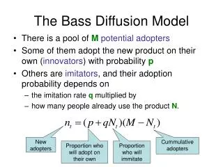
Assumptions of theBasic Bass Model • Diffusion process is binary (consumer either adopts, or waits to adopt) • Constant maximum potential number of buyers “m” (N) • Eventually, all m will buy the product • No repeat purchase, or replacement purchase • The impact of the word-of-mouth is independent of adoption time • Innovation is considered independent of substitutes • The marketing strategies supporting the innovation are not explicitly included
Adoption Probability over Time (a) 1.0 Cumulative Probability of Adoption up to Time t F(t) Introduction of product Time (t) (b) f(t) = d(F(t))dt Density Function: Likelihood of Adoption at Time t Time (t)
Number of Cellular Subscribers 9,000,000 5,000,000 1,000,000 1983 1 2 3 4 5 6 7 8 9 Years Since Introduction Source: Cellular Telecommunication Industry Association
Sales Growth Model for Durables (The Bass Diffusion Model) St = p ´ Remaining + q ´ Adopters ´ Potential Remaining Potential Innovation Imitation Effect Effect where: St = sales at time t p = “coefficient of innovation” q = “coefficient of imitation” # Adopters = S0 + S1 + • • • + St–1 Remaining = Total Potential – # Adopters Potential
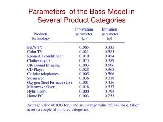
Parameters of the Bass Model in Several Product Categories Innovation Imitation Product/ parameter parameter Technology (p) (q) B&W TV 0.028 0.25 Color TV 0.005 0.84 Air conditioners 0.010 0.42 Clothes dryers 0.017 0.36 Water softeners 0.018 0.30 Record players 0.025 0.65 Cellular telephones 0.004 1.76 Steam irons 0.029 0.33 Motels 0.007 0.36 McDonalds fast food 0.018 0.54 Hybrid corn 0.039 1.01 Electric blankets 0.006 0.24 A study by Sultan, Farley, and Lehmann in 1990 suggests an average value of 0.03 for p and an average value of 0.38 for q.
Technical Specificationof the Bass Model The Bass Model proposes that the likelihood that someone in the population will purchase a new product at a particular time tgiven that she has not already purchased the product until then, is summarized by the following mathematical. Formulation Let: L(t): Likelihood of purchase at t, given that consumer has not purchased until t f(t): Instantaneous likelihood of purchase at time t F(t): Cumulative probability that a consumer would buy the product by time t Once f(t) is specified, then F(t) is simply the cumulative distribution of f(t), and from Bayes Theorem, it follows that: L(t) = f(t)/[1–F(t)] (1) Hazard Rate
Bass Model Math Differential Equation Solution to Differential Equation or
Bass Model Math: Estimation Bass Model can also be expressed as Sales = S(t) = m f(t) Cum. Sales = Y(t) = m F(t) Or, Estimate Directly with this: Run Regression a=p.m, b=(q-p) and c = -q/m. p = a/m q= -c.m
Why it Works--Saturation • S(t)=m[p+qF(t)][(1-F(t)] Gets Smaller and Smaller Gets Bigger and Bigger
Factors Affecting theRate of Diffusion Product-related • High relative advantage over existing products • High degree of compatibility with existing approaches • Low complexity • Can be tried on a limited basis • Benefits are observable Market-related • Type of innovation adoption decision (eg, does it involve switching from familiar way of doing things?) • Communication channels used • Nature of “links” among market participants • Nature and effect of promotional efforts
Some Extensions to theBasic Bass Model • Varying market potential As a function of product price, reduction in uncertainty in product performance, and growth in population, and increases in retail outlets. • Incorporation of marketing variables Coefficient of innovation (p) as a function of advertising p(t) = a + b ln A(t). Effects of price and detailing. • Incorporating repeat purchases • Multi-stage diffusion process Awareness è Interest è Adoption è Word of mouth
Some Extensions • Successive Generations of Technologies: • Generalized Bass Model: Includes Decision Variables: • Prices, Advertising
Successive Generations of Technology The Law of Capture-Migration&Growth • The Equations: Three Generations • S1,t=F(t1)m1[1-F(t2)] • S2,t=F(t2)[m2+F(t1)m1][1-F(t3)] • S3,t=F(t3){m3+F(t2)[m2+F(t1)m1]} • mi=incremental market potential for gen.i • ti=time since introduction of ith generation and F(ti) is Bass Model cumulative function and p and q are the same for each generation
Capture Law- DRAMSNorton and Bass: Management Science (1987)Sloan Management Review (1992)
What About Prices ? • The Generalized Bass Model • With Prices, Advertising, and other Marketing variables the curve is shifted with different policies but the shape stays the same. • Explain Why Adoption Curves Always Looks The Same Even Though Policies Vary Greatly: Model Must Reduce to Bass Model
Generalized Bass Model: Bass, Krishnan, andJain (1994) Marketing Science • A Higher Level Theory • Must Reduce as Special Case to Bass Model • Prices Fall Exponentially
The Bass Model (BM) and GBM • BM: f(t)/[1-F(t)]=[p+qF(t)] • GBM: f(t)/[1-F(t)]=x(t)[p+qF(t)] • where x(t) is a function of percentage change in price and other variables (eg: advertising) x(t) = 1+[(dPr(t)/dt)/Pr(t)]b1 + [(dADV(t)/dt)/ADV(t)]b2 X(t) = t+ Ln(Pr(t)/Pr(0)) b1 + Ln(ADV(t)/ADV(0)) b2
Impulse Response Comparison: GBM and “Current Effects” Model “Carry-Through” Effects for GBM
Some Applications • Guessing Without Data: • Satellite Television • Satellite Telephone (Iridium) • New LCD Projector • Wireless Telephone Adoption Around World and Pricing Effects • Projecting Worldwide PC Growth
Satellite TV Forecast-1993-”Guessing By Analogy” and Purchase Intentions • Use of “Adjusting Stated Intention Measures to Predict Trial Purchase of New Products: A Comparison …” Journal of Marketing Research (1989), Jamieson and Bass • “Guessing By Analogy”: Cable TV vs.Color TV
Projection of World-Wide PC Demand, 1999-2010-Data From Bill Gates, Newsweek 5-31-99
Bottom Line and Quotation “In Forecasting the Time of Peak It is Helpful to Know that a Peak Exists” By Frank Bass