Download
1 / 65
670 likes | 936 Views
Atmospheric Chemistry. Photochemical Pollutants - Ozone Formation and Degradation Global Warming Visibility. Dr. Steven Japar Ford Motor Co. – Retired March 29, 2005. TROPOSPHERIC CHEMISTRY John H. Seinfeld, Spyros N. Pandis, “Atmospheric Chemistry and Physics” (John Wiley & Sons, 1998).

E N D
Atmospheric Chemistry • Photochemical Pollutants - Ozone Formation and Degradation • Global Warming • Visibility Dr. Steven Japar Ford Motor Co. – Retired March 29, 2005
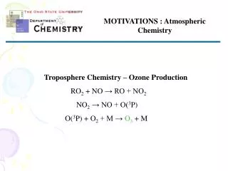
TROPOSPHERIC CHEMISTRYJohn H. Seinfeld, Spyros N. Pandis, “Atmospheric Chemistry and Physics” (John Wiley & Sons, 1998) Photochemical Cycle of NO2, NO and O3 • NO2 + hν (λ< 424 nm) NO + O (jNO2) • O + O2 + M O3 + M (k1) • O3 + NO NO2 + O2(k2) • d[NO2]/dt = k2[O3][NO] - jNO2[NO2 ] For O atoms, O3 (very reactive), invoke pseudo-steady-state approximation, i.e., rate of formation = equals rate of loss
d[O3]dt = k1[O][O2][M] - k2[O3][NO] ~ 0 • d[O]/dt = jNO2 [NO2 ] – k1[O][O2][M] ~ 0 jNO2[NO2] = k1[O][O2][M] • d[O3]dt = jNO2 [NO2] - k2[O3][NO] ~ 0 Photostationary state relationship [O3]ss = jNO2[NO2] /k2[NO]
Atmospheric Chemistry of Carbon Monoxide and NOx • O3 + hν O + O2 • O(1D) + O2 • O(1D) + M O + M • O + O2 + M O3 • O(1D) + H2O 2 OH • CO + OH CO2 + H • H + O2 + M HO2 + M • CO + OH + O2 CO2 + HO2 • HO2 + NO NO2 + OH
Atmospheric Catalytic Oxidation of CO CO + OH + O2 CO2 + HO2 HO2 + NO NO2 + OH NO2 + hν NO + O O + O2 + M O3 + M CO + 2O2 + hν CO2 + O3 • HO2,OH not consumed in this cycle • Net formation of O3: NO NO2 is accomplished by HO2 • The chain terminating step: OH + NO2 + M HNO3 + M
The Hydroxyl Radical • Most important reactive radical species in the atmosphere. • Measurements, theoretical estimates -- average tropospheric [OH] = • Daytime (summer) 5-10 x 106 molecules cm-3 • Daytime (winter) 1- 5 x 10⁶ • Nighttime <2 x 10⁵ • Nighttime reservoir OH + NO + M HONO + M • Early morning jump start HONO + hν OH + NO
Peroxyacyl Nitrates • CH3CHO + OH CH3CO + H2O • CH3CO + O2 + M CH3C(O)O2 + M • CH3C(O) O2 + NO CH3C(O)O + NO2 • CH3C(O)O CH3 + CO2 • CH3C(O)O2 + NO2 <==> CH3C(O)OONO2 Peroxyacetyl nitrate (PAN) CH3C=O OONO2
Peroxyacyl Nitrates • Lower troposphere -- relatively unreactive • Lifetime determined by thermal dissociation • PAN: ~ 30 minutes at 298 K; 8 hours at 273 K; months in upper troposphere • Upper troposphere – lifetime determined by photolysis, OH • Mechanism for long-range transport of reactive NOx
Hydrocarbon Oxidation in the Atmosphere CH4 + 4O2 + 2NO + OHHCHO + 2O3 + OH + 2NO2 + H2O CH3CH3 + 2NO + OH + O2CH3CHO + 2NO2 + OH C2H4 + OH + NO + 2O2 NO2 + 1.44 HCHO + 0.28 HOCH2CHO + OH
NOX/Hydrocarbon/Ozone Relationships in the Atmosphere Urban-Suburban O3: 100-400 ppb Rural O3: 50-120 ppb Marine O3: 20-40 ppb Remote O3: 20-40 ppb
Ozone Isopleths • Graphical representation of the dependence of O3 formation on initial [VOC] and [NOx] • Simple box model representation of the atmosphere • After initialization, nothing enters or leaves the box • Implications for Control of O3 All VOC/NOx regimes are not equal
Ridge line: low VOC/NOx vs. high VOC/NOx • Above ridge line Decreased [NOx] increased [O3] Decreased [VOC] decreased [O3] • Below ridge line: Decreased [NOx] decreased [O3] Decreased [VOC] no change in [O3] VOC-limited NOx-limited
Michigan Air Pollutionhttp://www.deq.state.mi.us/documents/deq-aqd-aqe-ozone-bumpdown-westmich.pdf • Air quality in Michigan has been improving since the mid-1980’s
Extinction Coefficient - bext • Measure of atmospheric transparency • Measure of the fraction of light energy lost from a collimated beam of energy E in traversing a unit thickness of atmosphere • The extinction coefficient has dimensions of inverse length (e.g., Mm-1)
bRayis light scattering by gas molecules known as Rayleigh scattering • Gas scattering is almost entirely attributable to oxygen and nitrogen molecules in the air. • It is unaffected by pollutant gases and is 12 x 10-6 m-1 (Mm-1) at the wavelength of 550nm at sea level. (Vr ~300 km) • bsp is light scattering by particles • Dominated by fine particles in the size range of 0.1~1.0 μm
bag is light absorption by gases • NO2 is the only common atmospheric gas that significantly absorbs light • bap is light absorption by particles • Absorption arises nearly entirely from elemental carbon particles
Dry • 0.1 2 µm diameter particles scatter the most light per unit mass. • Sulfates ~ two-thirds of the visibility reduction in the Appalachian Mts. • In southern California, nitrates are the greatest contributor to haze, with organic carbon also very important. Wet
Visual Range – Koschmieder Equation • Distant objects are perceived in terms of contrast against the background (usually the sky) • At increasing distances, both bright and dark objects fade and approach the horizon of the brightness • Apparent contrast relative to the horizon decreases
Initial object contrast (Co) = ratio of the object brightness minus the horizon brightness divided by the horizon brightness. • For a homogeneous atmosphere (pollutant concentration, sky brightness), the apparent contrast decreases with increasing object-observer distance; C = Coexp(bextx) bext is the extinction coefficient x is the observer-object distance.
For a large black object Co = -1; assume the contrast threshold for human perception is 0.02 0.02 = - exp(bextVr) and Vr = 3.912/bext • Pristine coastal air: Vr ~ 160-200 km • Remote continental air: Vr ~ 80-120 km • Urban Plume: Vr ~ 5-20 km
Smoke from multiple wildfires in Canada blanketed the eastern U.S. with a smoke plume nearly 200 miles wide, affecting air quality from New York to Washington D.C in July 2002. CREDIT: NASA/GSFC.
B. A. Schichtel, et al, Atmospheric Environment 35, 5205-5210 (2001) 1981-1985 1986-1990 1991-1995 bext derived from Vr
Visibility Trends in the Eastern U.S. Trends in improving visibility in the eastern U.S. correlate well with the decrease in SO2 emissions (precursor to particle sulfate in the atmosphere) in the U.S.
Air Emissions Trends - Continued Progress Through 2003 http://epa.gov/airtrends/econ-emissions.html National Air Pollutant Emissions Estimates for Major Pollutants
This image shows ocean-crossing aerosols as dust from the Sahara desert is carried over the Atlantic Ocean. Dust and pollution from Asia floats toward the Pacific Northwest. CREDIT: NASA/GSFC.
Definitions • Weather: Look out the window • High short-time variability • High, low pressure systems; meandering jet stream • High spatial variability (E. Lansing vs. Detroit) • Climate • Weather averaged over large areas (sub-continental global) and long time periods (decades centuries) • Recent climate change in Michigan?
What Determines Climate? • Physics and Chemistry of the Atmosphere • Greenhouse gases; aerosols • Feedbacks • Water Vapor and Clouds • The Sun • Interactions between Biosphere and Atmosphere • Natural Climate Variability
Facts • Since ~1800 • Earth has warmed 0.8oC (since 1880) • GHG atmospheric concentrations have increased • CO2: 280 ppm 370 ppm • CH4: 0.7 ppm 1.75 ppm • N2O: 270 ppb 320 ppb • Climate is controlled by the Greenhouse Effect
The Natural Greenhouse Effect Contribution to the Natural Greenhouse Water 90-95% Carbon Dioxide 5-7% Methane <1% Nitrous Oxide <1%
Physics and Chemistry of the Atmosphere • Greenhouse gas concentrations • Radiative forcings • Feedbacks • Chemistry, physics, meteorology • Water vapor and clouds
Atmospheric CO2 Concentrations Currently ~372 ppm
Aerosols/Particles • Major impact on climate • Atmospherically inhomogeneous, short lifetimes – unlike GHGs • Direct Effects – Fairly straight-forward • Particles scatter and absorb solar radiation • Light scattering cools (all particles) • Light absorption warms (primarily BC and iron-containing dust) • Indirect Effects – Very difficult to quantify • Cloud formation (condensation nuclei) • Cloud properties (water droplet size; cloud water content)
Feedbacks • 2x CO2 Direct warming ~0.5-1.0oC • Predictions ~5oC require positive climate system FEEDBACKS that amplify the direct warming from the extra GHGs. • Water vapor • Clouds • Inherent uncertainties in feedback mechanisms
Water Vapor and Clouds 8-Day Atmospheric Water Cycle • On average, clouds cover 40-45% of the Earth’s surface • Additional 2-3% cloud cover offsets warming from man-made GHG (+2.5 Wm-2) • Model grid scale requirements make it impossible to directly model clouds and their climate effects
Correlation Between Solar Cycle and Surface TemperatureCourtesy of George Wolff (GM) Dashed line is length of sun’s magnetic cycle..
Solar Hypothesis • Excellent correlation between solar activity and temperature for past 30,000 years • Solar activity greatest in last 8000 years S. Solanki, et al., Nature (28 Oct. 2004) • Change in directsolar forcing ~ 10% of the observed temperature variation • Solar/climate theory • High solar activity strengthens magnetic barrier which deflects cosmic particles away from earth (known) • Cosmic particles enhance cloud formation (limited recent data)
Global Average Radiative ForcingBaseline: Pre-Industrial Revolution TAR (IPCC, 2001)
Major Forcing Uncertainties • Black carbon • Very short-lived, strong solar energy absorber • As important as CO2? • Aerosol indirect forcing • Aerosols impact cloud formation, cloud characteristics • Offset much of the GHG warming? • Land use changes • Changes planetary surface albedo • Solar influence • An important warming component?
Natural Climate Variability • What do we “know”? • 140 years of “real” data, paleo-data, GCM predictions: +0.2-0.3oC • 100 Years of Consensus • Example: Sargasso Sea Temperatures Medieval Warm Epoch Little Ice Age
Natural Climate Variability • “Consensus” challenged in 1998 (IPCC 2001) by the Hockeystick • Minimized the importance of Medieval Warm Epoch; Little Ice Age – regional rather than global event
El Nino Australian Bureau of Meteorology
El Nino – hot and dry on west coast of Americas • La Nina – cold and rainy on west coast of Americas; intense drought in Australia • Global connections
Existing Issues • Radiative forcing – clouds, aerosols • Natural climate variability • CycleswithinCycleswithinCycles … • Ocean response - “Instantaneous” climate shifts freezing in the greenhouse? • Sea level – ice melt, thermal expansion; will the glaciers grow? • Carbon cycle - terrestrial sinks; deforestation • Land use • Extreme weather – floods, droughts, hurricanes • Regional climate change - “winners and losers”