EPS200: Atmospheric Chemistry
400 likes | 644 Views
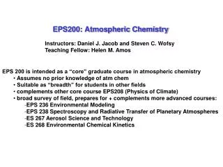
Instructors: Daniel J. Jacob and Steven C. Wofsy Teaching Fellow: Helen M. Amos. EPS200: Atmospheric Chemistry. EPS 200 is intended as a “core” graduate course in atmospheric chemistry Assumes no prior knowledge of atm chem Suitable as “breadth” for students in other fields

EPS200: Atmospheric Chemistry
E N D
Presentation Transcript
Instructors: Daniel J. Jacob and Steven C. Wofsy Teaching Fellow: Helen M. Amos EPS200: Atmospheric Chemistry • EPS 200 is intended as a “core” graduate course in atmospheric chemistry • Assumes no prior knowledge of atm chem • Suitable as “breadth” for students in other fields • complements other core course EPS208 (Physics of Climate) • broad survey of field, prepares for + complements more advanced courses: • EPS 236 Environmental Modeling • EPS 238 Spectroscopy and Radiative Transfer of Planetary Atmospheres • ES 267 Aerosol Science and Technology • ES 268 Environmental Chemical Kinetics
Point source Urban smog BIG PROBLEMS IN ATMOSPHERIC CHEMISTRY Ozone layer Visibility Disasters Climate Regional smog Biogeochemical cycles Acid rain GLOBAL > 1000 km LOCAL < 100 km REGIONAL 100-1000 km
GLOBAL OBSERVING SYSTEM FOR TROPOSPHERIC COMPOSITION Satellites Chemical transport models (CTMs) Surface networks Aircraft, ships CTMs solve coupled continuity equations for chemicals on global 3-D Eulerian grid: Emissions Transport Chemistry Aerosol processes Deposition Dx ~100 km Dz ~ 1 km
SEA-LEVEL PRESSURE CAN’T VARY OVER MORE THAN A NARROW RANGE: 1013 ± 50 hPa Consider a pressure gradient at sea level operating on an elementary air parcel dxdydz: P(x) P(x+dx) Pressure-gradient force Vertical area dydz Acceleration For DP = 10 hPa over Dx = 100 km, g ~ 10-2 m s-2 a 100 km/h wind in 3 h! Effect of wind is to transport air to area of lower pressure a dampen DP On mountains, however, the surface pressure is lower, and the pressure-gradient force along the Earth surface is balanced by gravity: P(z+Dz) P-gradient • This is why weather maps show “sea level” isobars; • The fictitious “sea-level” pressure at a mountain site assumes an air column to be present between the surface and sea level gravity P(z)
MASS ma OF THE ATMOSPHERE Mean pressure at Earth's surface: 984 hPa Radius of Earth: 6380 km Total number of moles of air in atmosphere: Mol. wt. of air: 29 g mole-1 = 0.029 kg mole-1
VERTICAL PROFILES OF PRESSURE AND TEMPERATUREMean values for 30oN, March Stratopause Tropopause
Barometric law (variation of pressure with altitude) • Consider elementary slab of atmosphere: P(z+dz) P(z) hydrostatic equation unit area Ideal gas law: Assume T = constant, integrate: Barometric law
ATMOSPHERIC TRANSPORT • Forces in the atmosphere: • Gravity • Pressure-gradient • Coriolis • Friction to R of direction of motion (NH) or L (SH) Equilibrium of forces: In vertical: barometric law In horizontal: geostrophic flow parallel to isobars gp P v P + DP gc In horizontal, near surface: flow tilted to region of low pressure gp P v gf P + DP gc
Air converges near the surface in low pressure centers, due to the modification of geostrophic flow under the influence of friction. Air diverges from high pressure centers. At altitude, the flows are reversed: divergence and convergence are associated with lows and highs respectively
HOT COLD COLD THE HADLEY CIRCULATION (1735): global sea breeze • Explains: • Intertropical Convergence Zone (ITCZ) • Wet tropics, dry poles • General direction of winds, easterly in the tropics and westerly at higher latitudes • Hadley thought that air parcels would tend to keep a constant angular velocity. • Meridional transport of air between Equator and poles results in strong winds in the longitudinal direction. • …but this does not account for the Coriolis force correctly.
TODAY’S GLOBAL INFRARED CLOUD MAP (intellicast.com) shows Intertropical Convergence Zone (ITCZ) as longitudinal band near Equator Bright colors indicate high cloud tops (low temperatures) Today
TROPICAL HADLEY CELL • Easterly “trade winds” in the tropics at low altitudes • Subtropical anticyclones at about 30o latitude
500 hPa (~6 km) CLIMATOLOGICAL WINDS IN JANUARY:strong mid-latitude westerlies
500 hPa (~5 km) CLIMATOLOGICAL WINDS IN JULYmid-latitude westerlies are weaker in summer than winter
y x P u P + DP ZONAL GEOSTROPHIC FLOW AND THERMAL WIND RELATION Geostrophic balance: Thermal wind relation:
ZONAL WIND: VARIATION WITH ALTITUDE follows thermal wind relation
TIME SCALES FOR HORIZONTAL TRANSPORT(TROPOSPHERE) 1-2 months 2 weeks 1-2 months 1 year
What is buoyancy? Dust transport over the Pacific, April 21-25, 1998 R. Husar
TRANSPORT OF ASIAN DUST TO NORTH AMERICA Clear day April 16, 2001: Asian dust! Glen Canyon, AZ Mean April 2001 PM concentrations measured by MODIS
GLOBAL TRANSPORT OF CARBON MONOXIDE (CO) Sources of CO: Incomplete combustion (fossil fuel, biofuel, biomass burning), oxidation of VOCs Sink of CO: atmospheric oxidation by OH radical (lifetime ~ 2 months) MOPITT satellite observations of CO concentrations at 500 hPa (~6 km)
OBSERVATION OF CO FROM AIRS SATELLITE INSTRUMENT AIRS CO data at 500 hPa (W.W. McMillan) Averaging kernels for AIRS retrieval
“Lapse rate” = -dT/dz ATMOSPHERIC LAPSE RATE AND STABILITY Consider an air parcel at z lifted to z+dz and released. It cools upon lifting (expansion). Assuming lifting to be adiabatic, the cooling follows the adiabatic lapse rateG : z G = 9.8 K km-1 stable z unstable • What happens following release depends on the local lapse rate –dTATM/dz: • -dTATM/dz > Ge upward buoyancy amplifies initial perturbation: atmosphere is unstable • -dTATM/dz = Ge zero buoyancy does not alter perturbation: atmosphere is neutral • -dTATM/dz < Ge downward buoyancy relaxes initial perturbation: atmosphere is stable • dTATM/dz > 0 (“inversion”): very stable ATM (observed) inversion unstable T The stability of the atmosphere against vertical mixing is solely determined by its lapse rate.
WHAT DETERMINES THE LAPSE RATE OF THE ATMOSPHERE? • An atmosphere left to evolve adiabatically from an initial state would eventually tend to neutral conditions (-dT/dz = G ) at equilibrium • Solar heating of surface and radiative cooling from the atmosphere disrupts that equilibrium and produces an unstable atmosphere: z z z final G ATM G ATM initial G T T T Initial equilibrium state: - dT/dz = G Solar heating of surface/radiative cooling of air: unstable atmosphere buoyant motions relax unstable atmosphere back towards –dT/dz = G • Fast vertical mixing in an unstable atmosphere maintains the lapse rate to G. • Observation of -dT/dz = Gis sure indicator of an unstable atmosphere.
IN CLOUDY AIR PARCEL, HEAT RELEASE FROM H2O CONDENSATION MODIFIES G Wet adiabatic lapse rate GW = 2-7 K km-1 z T RH 100% GW “Latent” heat release as H2O condenses GW = 2-7 K km-1 RH > 100%: Cloud forms G G = 9.8 K km-1
4 3 Altitude, km 2 1 0 -20 -10 0 10 20 30 Temperature, oC cloud boundary layer
SUBSIDENCE INVERSION typically 2 km altitude
DIURNAL CYCLE OF SURFACE HEATING/COOLING:ventilation of urban pollution z Subsidence inversion PBL depth MIDDAY 1 km G Mixing depth NIGHT 0 MORNING T NIGHT MORNING AFTERNOON
VERTICAL PROFILE OF TEMPERATUREMean values for 30oN, March Radiative cooling (ch.7) - 3 K km-1 Altitude, km 2 K km-1 Radiative heating: O3 + hn e O2 + O O + O2 + M e O3+M heat Radiative cooling (ch.7) Latent heat release - 6.5 K km-1 Surface heating
BAROCLINIC INSTABILITY q3 > q2 z > q1 Buoyant vertical motion Is possible even when 0 latitude Dominant mechanism for vertical motion in extratropics
FIRST-ORDER PARAMETERIZATION OF TURBULENT FLUX Time-averaged envelope Near-Gaussian profile • Observed mean turbulent dispersion of pollutants is near-Gaussian eparameterize it by analogy with molecular diffusion: z Instantaneous plume Source <C> Turbulent diffusion coefficient • Typical values of Kz: 102 cm2s-1 (very stable) to 107 cm2 s-1 (very unstable); mean value for troposphere is ~ 105 cm2 s-1 • Same parameterization (with different Kx, Ky) is also applicable in horizontal direction but is less important (mean winds are stronger)
TYPICAL TIME SCALES FOR VERTICAL MIXING • Estimate time Dt to travel Dz by turbulent diffusion: tropopause (10 km) 10 years 5 km 1 month 1 week 2 km “planetary boundary layer” 1 day 0 km