Production Function

1. Production Function

2. Production Function Production: Any activity leading to value addition – Transformation of inputs into output Q= f (L,K)

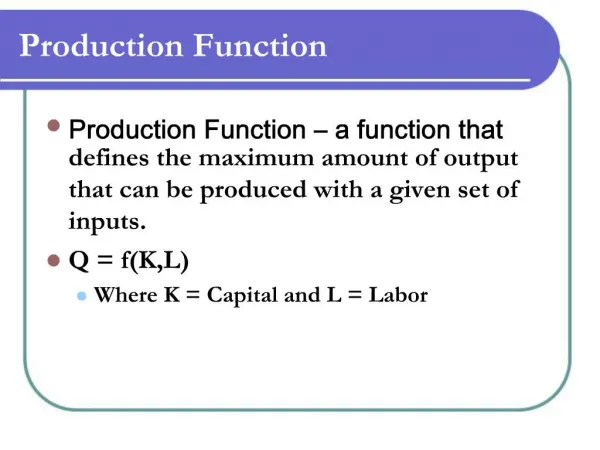
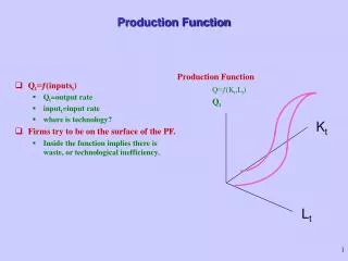
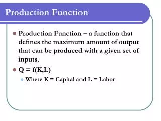
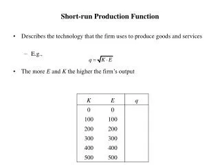
3. Production Function Short term : Time when one input (say, capital) remains constant and an addition to output can be obtained only by using more labour. Long run: Both inputs become variable.

4. Production Function Production process is subject to various phases- Laws of production state the relationship between output and input. .

5. Laws of production Short run : Relationship between input and output are studied by varying one input , others being held constant. Law of Variable Proportions brings out relationship between varying proportions of factor inputs and output

6. Laws of production Long run: Production function is subject to different phases described under the Law of Returns to Scale – Studied assuming that all factor inputs are variable.

7. Law of Variable Proportions Law of Variable Proportions (Short run Law of Production) Assumptions: • One factor (say, L) is variable and the other factor (say, K) is constant • Labour is homogeneous • Technology remains constant • Input prices are given

8. Law of Variable Proportions

9. Law of Variable Proportions Panel A TP rises at an increasing rate till the employment of the 5th worker. Beyond the 6th worker until 10th worker TP increases but rate of increase begins to fall TP turns negative from 11th worker onwards. This shows Law of Diminishing Marginal returns Total Product TPl Total product Total Product Labour

10. Law of Variable Proportions Panel B Panel B represents Marginal and average productivity curves of labour AP/MP APL MPL MPL labour

11. Law of Variable Proportions Increasing Returns- Stage I: TPlincreases at an increasing rate. Fixed factor (K) is abundant and variable factor is inadequate. Hence K gets utilised better with every additional unit of labour

12. Stage II- TPl continues to increase but at a diminishing rate. stage III- TPl begins to decline –Capital becomes scarce as compared to variable factor. Hence over utilisation of capital and setting in of diminishing returns Causes of 3 stages: Indivisibility and inelasticity of fixed factor and imperfect substitutability between K and L

13. Law of Variable Proportions Significance of Law of Diminishing Marginal Returns: • Empirical law, frequently observed in various production activities • Particularly in agriculture where natural factors (say land), which play an important role, are limited. • Helps manager in identifying rational and irrational stages of operation

14. Law of Variable Proportions • It provides answers to questions such as: a) How much to produce? b) What number of workers (and other variable factors) to employ in order to maximize output In our example, firm should employ a minimum of 7 workers and maximum of 10 workers (where TP is still rising)

15. Law of Variable Proportions • Stage III has very high L-K ratio- as a result, additional workers not only prove unproductive but also cause a decline in TPl. • In Stage I capital is presumably under-utilised. • So a firm operating in Stage I has to increase L and that in Stage III has to decrease labour.

16. Law of Returns to Scale In the long run, all factors are variable. • Production can be increased by adding both L and K. • Relationship between inputs and output is depicted in the form of isoquant curves. • Isoquant curves represent different combinations of K and L that lead to the same level of output.

17. ISOQUANT CURVES Y IQ300 Units of K IQ200 IQ100 o X Units of L

18. Law of Returns to Scale Isocost line: • Assume that labour costs Rs.10 per unit and capital, Rs. 7 per unit. • Suppose the company has a budget of Rs. 70. • It can buy 7 units of labour (with no capital), or 10 units of K (with no labour), or some in-between combination. • By joining the two extreme points we get an isocost line

19. Law of Returns to Scale Y 10 Units of K Isocost X o 7 Units of L

20. Law of Returns to Scale Producer has a constraint- namely, budget. Producer attains equilibrium when he reaches highest attainable level of output. Y Y Capital Q3=300 Q2=200 B Q1=100 10019 X O Labour

21. Law of Returns to Scale • Point of tangency between isoquant and isocost is the point of least cost combination of inputs. • At point B, labour and capital are combined in a proportion that maximises the output for a given budget.

22. Law of Returns to Scale ε= Δq/ q ÷ Δn /n where Δq/ q indicates proportionate change in output Δn /n indicates proportionate change in input If ε>1, then we have increasing returns to scale ε=1, then we have constant returns to scale ε<1, then we have decreasing returns to scale

23. Law of Returns to Scale Y Expansion Path Q140 Firm is subject to increasing, Constant and Decreasing returns to scale. Explanation for these phases is provided Through concepts Called economies And diseconomies Of scale. G Q120 F K E Q100 D Q80 C Q60 B B Q40 A Q 20 o X L

24. ECONOMIES OF SCALE • ECONOMIES OF SCALE are advantages enjoyed by a firm from large scale production. Causes of increasing returns to scale • Internal and external

25. INTERNAL ECONOMIES INTERNAL: Those advantages and disadvantages that accrue to the firm as a result of its scale of operation Indivisibilities- if some of the factors are indivisible, then it would be technically and economically undesirable to use the indivisible factor for a smaller scale of production e.g., Can’t use a conveyor belt to unload a small truck, but need one for unloading a train or ship

26. INTERNAL ECONOMIES Dimensional economies • A mere change in the size of capital can lead to a change in output which is proportionately more than the cost of enlarged input. e.g., Doubling the diameter of a pipeline more than doubles the water flow without doubling the cost; doubling the dimensions of a ship more than doubles its capacity without doubling costs

27. INTERNAL ECONOMIES • Specialisation- In large scale production, a process can be broken into sub processes - specialised labour and specialised machines lead to increase in productivity and decrease in average cost of production. • Managerial economies • Commercial economies-bulk purchases

28. INTERNAL ECONOMIES • Financial economies -Lower rate of interest, liberal terms and conditions because of reputation individual investors also like to invest money. • Risk bearing economies: • Diversification of output, markets and sources of supply

29. INTERNAL DISECONOMIES Internal Diseconomies • Effective supervision no longer possible • Unwieldy administration and ego clashes • Industrial unrest • Problems of re-conversion, storage and standing costs in case of stoppage of work or lack of demand

30. External Economies of Scale External Economies of Scale Arise out of sharing and cooperation received from other firms in a given industry.

31. External Economies of Scale Economies of concentration • Supply of skilled labour in a region • Common services • Specialised institutions like training schools and research centres (Indian School of mines in Dhanbad), • Reputation of a region

32. External Economies of Scale Economies of Information • Trade associations, journals, seminars • Economies of disintegration • An ancillary firm may specialise in the production of only one part • Waste and byproducts of all firms in the industry may be dealt with by a specialised firm.

33. External Diseconomies of Scale • As firms expand along with expansion of the industry, after a point economies turn into diseconomies • Excessive concentration leads to bottlenecks and diseconomies • Most firms experience these phases but some continue to defy these laws due to innovations and technological progress.

34. Economies of Scope • Lowering of costs that a firm experiences when it produces more than one product together rather than each alone • A smaller airline can profitably extend into cargo services, thereby lowering the cost of each service • Using bye products to make something instead of throwing it away. • Management should be alert to such possibilities.

35. Learning Curve • As a firm gains experience in the production of a commodity or service, AC often declines. • Learning Curve shows the decline in the average input cost of production with the rising cumulative total output over time. • Eg, 1000 hours to assemble 100th aircraft, but only 700 hours to assemble the 200th .as managers and workers become more efficient as they gain production experience.

37. Case study: Masterji’s Grocery Shop Masterji’s shop is very popular and stocks all kinds of goods- from rice and wheat to processed food, imported chocolates and cheese. There is a small section which has a photocopying machine and a STD booth. Masterji runs the shop with the help of his children.

38. Case study: Masterji’s Grocery Shop • The family noticed that the number of shoppers varied between times and days (See table) • During weekdays, masterji could manage with his children, but not in week ends.

39. Case study: Masterji’s Grocery Shop • Sunday morning buyers were ‘ value crowd’- bulk buyers, spent extra on something new and attractive but wanted a pleasant experience and were upset at the overcrowded shop • At certain times there were not many shoppers

40. Case study: Masterji’s Grocery Shop • Masterji employed 3 assistants during week ends, but that did not solve the problem as the shop had a small floor area and only one billing machine 1.Can you explain masterji’s problem in terms of law of variable proportions? 2. Pl. suggest in detail how masterji can improve the functioning of the shop.

41. Measuring Productivity • US Bureau of Labor Statistics has been conducting studies of output per hour in individual industries as well as overall economy since 1800s- earlier because of apprehensions of human labor being displaced- this fear of unemployment was replaced by concern for making the most efficient use of labour in 1920s and 30s- In recent years interest in productivity measurement and enhancement has grown because it is recognised as an important indicator of economic growth.

42. Labor productivity: Ratio of output per worker hour. Improvements in worker productivity • Multifactor productivity: Output is related to combined inputs of labor, capital and intermediate purchases. • Advances in productivity reflect the ability to produce more output per input