The Production Function
Ch 6 – Costs. The Production Function. It takes factors of production to produce a good or service – no matter what the good is. Factors of production – Resource inputs used to produce goods and services, such as land, labor, capital, enterprise. The Production Function.

The Production Function
E N D
Presentation Transcript
Ch 6 – Costs The Production Function • It takes factors of production to produce a good or service – no matter what the good is. • Factors of production – Resource inputs used to produce goods and services, such as land, labor, capital, enterprise.
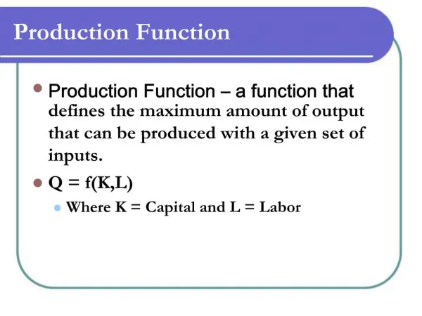
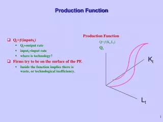
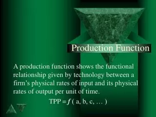
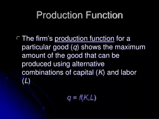
The Production Function • Production function - technological relationship expressing the maximum quantity of a good attainable from different combinations of factor inputs. • Purpose - to tell us just how much output we can produce with varying amounts of factor inputs. • Productivity – output per unit
A Production Function Y = f(L, K)
Efficiency • The production function represents the maximum technical efficiency. • Efficiency (technical) - maximum output of a good from the resources used in production.
Short-Run Constraints • Short-run – at least one input is fixed (does not change as quantity changes). • Labor (L) is usually the variable input being added to fixed inputs (K).
55 G H F E I 50 D 45 40 35 C 30 Jeans Output (pairs per day) 25 20 B 15 10 5 0 A 1 2 3 4 5 6 7 8 Labor Input (machine operators per day) Short-Run Production Function Total output (per day) Output rates depend on input levels
Marginal Productivity • Marginal physical product(MPP) - change in total output that results from employment of one additional unit of input.
G H F E I D C B c d b e g f h A a i Marginal Physical Product 55 Total output (per day) 50 45 40 + 10 jeans 35 30 Third worker Jeans Output (pairs per day) 25 20 Marginal physical product (per worker) 15 10 5 0 3 4 5 1 2 6 7 8 Labor Input (machine operators per day)
Law of Diminishing Marginal Returns • Law of diminishing marginal returns - the marginal physical product of a variable input declines as more of it is employed with a given quantity of other (fixed) inputs.
G H F E I D C B c d b e g f h A a i Diminishing Marginal Returns 55 Total output (per day) 50 45 40 35 30 Jeans Output (pairs per day) 25 20 Marginal physical product (per worker) 15 10 5 0 3 4 5 1 2 6 7 8 Labor Input (machine operators per day)
Resource Costs • A production function tells us how much a firm can produce but not how much it should produce. • The most desirable rate of output is the one that maximizes total profit. • Profit - The difference between total revenue and total cost.
Marginal Resource Cost • Marginal cost(MC) is the increase in total costs associated with a one unit increase in production.
Marginal Resource Cost • Whenever MPP is increasing, the marginal cost of producing a good must be falling. • If marginal physical product declines, marginal cost increases.
24 1.20 c 1/g 1.00 20 16 0.80 b Diminishing marginal physical product Rising marginal cost 12 0.60 Marginal Physical Product Additional Labor Cost d 1/f 8 0.40 1/e e 4 0.20 1/d f 1/b 1/c g h 0 1 2 3 4 5 6 7 8 0 1 2 3 4 5 6 7 i Labor Input Labor Input Falling MPP Implies Rising Marginal Cost Diminishing marginal productivity implies . . . Rising marginal cost
Costs The dollar costs of production are directly related to the underlying production function. • Total cost - market value of all the resources used to produce a good or service. • Fixed costs - costs of production that do not change when the rate of output is altered, such as the cost of basic plant and equipment. • Variable costs - costs of production that change when the rate of output is altered, such as labor and material costs.
Total Cost • How fast total costs rise depends on variable costs only. • Total cost is equal to the fixed costs when output is zero. • There is no way to avoid fixed costs in the short run. TC = FC + VC
$1,200 1,100 1,000 900 800 700 G 600 Production Costs (dollars per day) 500 400 B 300 A 200 100 0 15 30 45 60 75 Rate of Output (pairs of jeans per day) The Cost of Jeans Production Total cost include variable and fixed costs Total cost Variable costs Variable costs Fixed costs
Average Costs • Average total cost(ATC) - total cost divided by the quantity produced in a given time period.
Average Costs • Average fixed cost(AFC) - total fixed cost divided by the quantity produced in a given time period.
Average Costs • Average variable cost(AVC) - total variable cost divided by the quantity produced in a given time period. ATC = AFC + AVC
$24 I 20 ATC J 16 O K N L M Costs (dollars per pair) 12 8 AVC 4 AFC 0 10 20 30 40 50 Rate of Output (pairs per day) Average Costs
Shape of Cost Curves Falling AFC • As the rate of output increases, AFC decreases as the fixed cost is spread over more output. • Any increase in output lowers average fixed cost. Rising AVC • AVC will eventually rise as the rate of output increases. • AVC rises because of diminishing returns in the production process.
Shape of Cost Curves U-Shaped ATC • The initial dominance of falling AFC, combined with the later resurgence of rising AVC, is what gives the ATC curve its characteristic U shape. Minimum ATC • The bottom of the U-shaped average total cost curve represents the minimum average total costs. • It identifies the lowest possible opportunity costs to produce the product. • Profit aren’t necessarily maximized where average total costs are minimized.
Marginal Cost • Marginal cost - the change in total costs associated with one more unit of output. • Diminishing returns in production cause marginal costs to increase as the rate of output is expanded.
v u t s q r p Marginal Cost $35 30 Added output is increasingly expensive 25 20 15 10 5 10 20 30 40 50 Rate of Output (pairs per day)
A Cost Summary • The marginal cost curve always intersects the ATC curve at its lowest point. If MC > ATC, ATC is increasing If MC < ATC, ATC is decreasing If MC = ATC, ATC at minimum
$32 28 24 20 16 Cost (dollars per unit) 12 8 4 0 1 2 3 4 5 6 7 8 9 Rate of Output (units per time period) Basic Cost Curves MC ATC AVC m AFC n
Economic vs. Accounting Costs • Accountants typically count dollar costs only and ignore any resource use that doesn’t result in an explicit dollar cost. • Economists consider implicit costs as well as explicit costs to be part of the total costs of production.
Economic vs. Accounting Costs • Explicit costs - payments made for the use of a resource. • Implicit costs - value of resources used, even when no direct payment is made (opportunity costs).
Economic vs. Accounting Cost • Economic cost - value of all resources used to produce a good or service; opportunity cost.
Long-Run Costs • The short-run is characterized by costs that cannot be changed (fixed costs). • There are no fixed costs in the long-run. • Thelongrun is a period of time long enough for all inputs to be varied (no fixed costs).
ATC1 ATC2 ATC3 Costs (dollars per pair) Long-run average total cost (LATC) 0 40 a 60 b c Rate of Output (pairs of jeans per day) Long-Run Average Costs • The long-run cost curve is a summary of our best short-run cost possibilities.
Long-Run Marginal Costs • The long-run marginal costs curve intersects our long-run cost curve at its lowest point.
LMC ATC2 Costs (dollars per pair) LATC m2 0 q2 Rate of Output (jeans per day) Long-Run Costs with Unlimited Options The long-run marginal costs curve intersects our long-run cost curve at its lowest point.
Economies of Scale • In long run, a firm can decide to use one large plant or several smaller plants to produce a given amount of output. • Economies of scale - reductions in minimum average costs that come about through increases in the size (scale) of plant and equipment.
Economies of Scale • Constant returns to scale - increases in plant size do not affect minimum average cost – minimum per-unit costs are identical for small plants and large plants.
Economies of Scale • Efficiency and size do not necessarily go hand in hand. • Diseconomiesofscale occur when an increase in plant size results in reducing operating efficiency.
Diseconomies of scale Constant returns to scale Economies of scale ATC3 ATC1 ATCS ATCS ATCS m3 ATC2 COST (dollars per unit) m1 m2 c c c 0 QM 0 QM 0 QM RATE OF OUTPUT (units per period) RATE OF OUTPUT (units per period) RATE OF OUTPUT (units per period) Economies of Scale
When the production function shifts up Cost curves shift down ATC1 ATC2 TOTAL OUTPUT (units per time period) COST (dollars per unit) MC1 MC2 Resource Inputs (dollars per unit) Rate of Output (units per time period) Improvements in Productivity Reduce Costs