Production Function,
Production Function,. SARBJEET KAUR Lecturer in Economics GCCBA-42 ,Chandigarh Email:kamalsingh84@gmail.com.

Production Function,
E N D
Presentation Transcript
Production Function, SARBJEET KAUR Lecturer in Economics GCCBA-42 ,Chandigarh Email:kamalsingh84@gmail.com
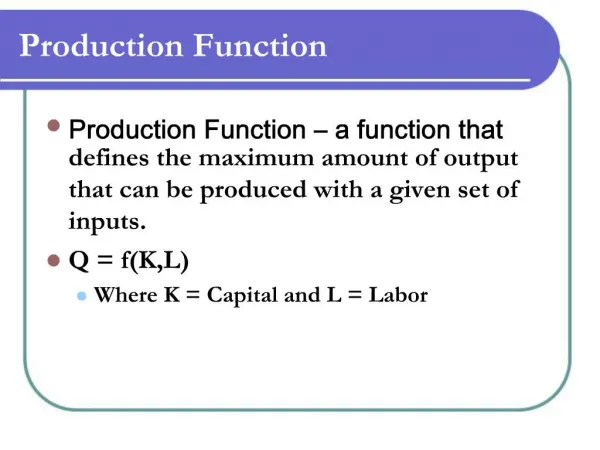
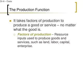
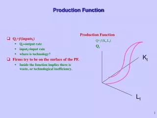
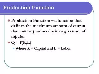
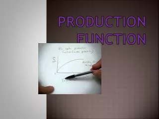
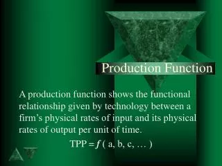
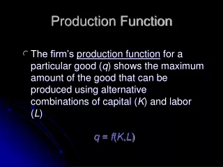
Production Function: Production of goods requires resources or inputs. These inputs are called factors of production named as land, labor, capital and organization. A rational producer is always interested that he should get the maximum output from the set of resources or inputs available to him. He would like to combine these inputs in a technical efficient manner so that he obtains maximum desired output of goods. The relationship between the inputs and the resulting output is described as production function. A production function shows the relationship between the amounts of factors used and the amount of output generated per period of time. Production functionestablishes a physical relationship between output and inputs. It describes what is technical feasible when the firm uses each combination of input. The firm can obtain a given level of output by using more labor and less capital or more capital and less labor. Production function describes the maximum output feasible for a given set of inputs in technical efficient manner.
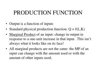
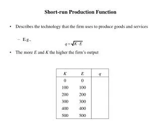
Short run and Long Run: The analysis of production function is generally carried with reference to time period which is called short period and long period. The short run is a period of time in which only one input (say labor) is allowed to vary while other inputs land and capital are held fixed. In the long run al the factors of production are variable. The long run is the lengthy period of time during with all inputs can be varied. There are no fixed output in the long run. All factors of production are variable inputs. • In the short run, therefore, production can be increased with one variable factor and other factors remaining constant. In the short run, the law of variable proportion governs the production behavior of a firm. The law of variable proportion shows the direction and rate of change in the output of firm when the amount of only one factor of production is varied while other factor of production are held constant. The law of variable proportion passes mainly through two phases, (i) Increasing Returns and (ii) Diminishing Returns.
Law of Variable Proportions (Short Run Analysis of Production): • There were three laws of returns mentioned in the history of economic thought up till Alfred Marshall's time. These laws were the laws of increasing returns, diminishing returns and constant returns. Dr. Marshall was of the view that the law of diminishing returns applies to agriculture and the law of increasing returns to industry. Much time was wasted in discussion of this issue. However, it was later on recognized that there are not three laws of production. It is only one law of production which has three phases, increasing, diminishing and negative production. This general law of production was named as the Law of Variable Proportions or the Law of Non-Proportional Returns. • The Law of Variable Proportions which is the new name of the famous law of Diminishing Returns has been defined by Stigler in the following words. "As equal increments of one input are added, the inputs of other productive services being held constant, beyond a certain point, the resulting increments of produce will decrease i.e., the marginal product will diminish According to Samuelson, "An increase in some inputs relative to other fixed inputs will in a given state of technology cause output to increase, but after a point, the extra output resulting from the same addition of extra inputs will become less".
Causes of Initial Increasing Returns: • The phase of increasing returns starts when the quantity of a fixed factor is abundant relative to the quantity of the variable factor. As more and more units of the variable factor are added to the constant quantity of the fixed factor, it is more intensively and effectively used. This causes the production to increase at a rapid rate. Another reason of increasing returns is that the fixed factor initially taken is indivisible. As more units of the variable factor are employed to work on it, output increases greatly due to fuller and effective utilization of the variable factor. • (ii) Stage of Diminishing Returns. This is the most important stage in the production function. In stage 2, the total production continues to increase at a diminishing rate until it reaches its maximum point (H) where the 2nd stage ends. In this stage both the • marginal product (MP) and average product of the variable factor are diminishing but are positive.
Causes of Diminishing Returns: • The 2nd phase of the law occurs when the fixed factor becomes inadequate relative to the quantity of the variable factor. As more and more units of a variable factor are employed, the marginal and average product decline. Another reason of diminishing returns in the production function is that the fixed indivisible factor is being worked too hard. It is being used in non-optima! proportion with the variable factor, Mrs. J. Robinson still goes deeper and says that the diminishing returns occur because the factors of production are imperfect substitutes of one another. • (iii) Stage of Negative Returns. In the 3rd stage, the total production declines. The TP, curve slopes downward (From point H onward). The MP curve falls to zero at point L2 and then is negative. It goes below the X axis with the increase in the use of • variable factor (labor).
Causes of Negative Returns: • The 3rd phases of the law starts when the number of a variable, factor becomes, too excessive relative, to the fixed factors, A producer cannot operate in this stage because total production declines with the employment of additional labor.arational producer will always seek to produce in stage 2 where MP and AP of the variable factor are diminishing. At which particular point, the producer will decide to produce depends upon the price of the factor he has to pay. The producer will employ the variable factor (say labor) up to the point where the marginal product of the labor equals the given wage rate in the labor market.
Returns to Scale The laws of returns to scale explain the behavior of output in response to a proportional and simultaneous change in inputs. Increasing inputs proportionately and simultaneously is, in fact, an expansion of the scale of production.
When a firm increases both the inputs proportionately, there are three possibilities • Total output may increase more than proportionately • Total output may increase proportionately • Total output may increase less than proportionately
Accordingly, there are three kinds of return to scale • Increasing returns to scale • Constant returns To Scale • Decreasing returns to scale
It refers to changes in output resulting from a proportional change in all inputs (where all inputs increase by a constant factor). If output increases by that same proportional change then there are constant returns to scale (CRS). If output increases by less than that proportional change, there are decreasing returns to scale (DRS).