Download
1 / 19
190 likes | 307 Views
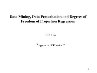
Data Mining, Data Perturbation and Degrees of Freedom of Projection Regression T.C. Lin * appear in JRSS series C. Canadian lynx data gives the annual record of the Canadian lynx trapped in the Mackenzie River district of the North-West Canada for the period 1821-1934. (n=114)

E N D
Data Mining, Data Perturbation and Degrees of Freedom of Projection Regression • T.C. Lin • * appear in JRSS series C
Canadian lynx data gives the annual record of the Canadian lynx trapped in the Mackenzie River district of the North-West Canada for the period 1821-1934. (n=114) • Some about this data set • is a fairly noisy set of field data. • has nonlinear and no Gaussian characteristics (see Tong, 1990). • has been used as a benchmark to gauge the performance of various time series methods. (cf. Campbell and Walker (1977), Tong (1980, 1990), Lim (1987))
Nowadays the same data set is used routinely in the formulation, selection, estimation, diagnostics and prediction of statistical models. • Parametric: • Linear: AR, MA, ARMA • Nonlinear: SETAR, ARCH,... • Nonparametric* • Most general: Xt = f (Xt-i1, …, Xt-ip) + et • Additive: Xt = f 1(Xt-i1)+...+fp (Xt-ip ) + et (ADD) • PPR:Y = β0+ΣKk=1βkfk(a’kX)+e, • *The selection, estimation are usually based on the smoothing, back fitting, BRUTO, ACE, Projector, etc. • (Hastie, 1990)
Questions: • Is it possible to compare performances of such models? • (/ Can nonparametric methods produce models with better predictive power than the parametric methods?) • What is the degrees of freedom(df) of a model? • (/ How can one access and adjust for the impact of data mining?) • While no universal answer can be expected, a data perturbation procedure (Wong and Ye, 1996) is used here to assess and adjust the impact of df to each fitted model.
Why Data Mining? The theory of statistical inference is based on the assumption that the model for the data is given a priori.i.e., x1,...,xn ~ p(x|Θ), p(x|Θ) is the known distribution with unknown parametersΘ. But in practice this assumption is not tenable since the model is seldom formulated using the subject-matter knowledge or data-free procedures. Consequently, over fitting or data mining occurs frequently in the modern data analysis environment.
How to count the df? • Parametric • df = # of parameters in the model. • Nonparametric • df is at the heart of the problem of assessing the impact of data mining. • Example 1. Y=WY, df = tr (W), see Hastie and Tibshirani (1990). • Example 2. df = tr (H), introduced later.
Idea of data perturbation: Intuitively and ideally, any estimated model should be validated using a new data set. It can be viewed as a method of generating new data that is close to the observed response Y (a generalization of the Breiman's little bootstrap method) . we would like to have, => Effective degrees of freedom (EDF) = tr(H) = hii
Table 1. MSE & SD of five models fitted to lynx data About SD: Fit the same class of models to the first 100 obs., keeping the last 100 for out-of-sample predictions. SD = the standard deviation of the multi-step ahead prediction errors.
Models for the lynx data. ◆Model 1: Moran’s AR(2) model Xt = 1.05 + 1.41 Xt-1 - 0.77Xt-2 + et, et ~ WN (0,0.04591). ◆Model 2: Tong’s SETAR (2;7,2) model 0.546+1.032Xt-1-0.173Xt-2+0.171 Xt-3 -0.431Xt-4+0.332X-0.284Xt-6 Xt= +0.210Xt-7+et(1) if Xt-2≦3.116 2.632+1.492Xt-1-1.324Xt-2+et(2) if Xt-2>3.116 var(et(1))= 0.0259, var(et(2))= 0.0505. (Pooled var = 0.0358).
BRUTO Algorithm (see HT 90) is a forward model selection procedure using a modified GCV, defined by to choose the significant variables and their smoothing parameters.
K = 5 (number of potential variable) • Model 3: ADD(1,2) Xt = 1.07 + 1.37 Xt-1 + s (Xt-2, 3) + et, • where • et ~ WN(0,0.0455) • s(x, d) stands for a cubic smoothing spline with df = d fitted to a time series x.
K=10: • Model 4: ADD(1,2,9) • Xt = 0.61 + 1.15 Xt-1 + s(Xt-2,3) + s(Xt-9,3) + et, • where et ~ WN (0,0.0381).
What is PPR (Projection pursuit )? • Let • Xt-1=(Xt-i1, Xt-i2, ..., Xt-ip)' be a random vector and • a1, a2, ... denote some p-dimensional unit ``direction" vectors. • The PPR are additive models of linear combinations of past values, • Xt = ΣKk=1fk*(a’k Xt-1)+et • = β0+ΣKk=1βkfk(a’k Xt-1)+et.
Model 5: PPR • Because of model 4 and for simplicity we take Xt = (xt-1, xt-2, xt-9)' as the covariate. Using the PPR algorithm , we have • and MSE = 0.0194 .
Data Perturbation Procedure: • For an integer m > 1 (the Monte Carlo sample size), generateδ1, ...,δm as i.i.d. N(0, t2In) where t > 0 and In is the n×n identity matrix. • Use the ``perturbed" data Y +δj, to re-compute (refit) • For i =1,2, ..., n, the slope of the LS line fitted to ( (Yi +δij), δij), j=1, ..., m, gives an estimate of hii.
Conclusion: The comparison and our findings bring home the danger of not accounting for the impact of data mining. Evidently, extensive data mining yields models and estimates that are too faith to the data with small (in-sample) prediction error and yet considerable loss in out-of-sample prediction accuracy.