Download
1 / 27
270 likes | 740 Views
Automatic Synthesis Using Genetic Programming of Improved PID Tuning Rules Martin A. Keane Econometrics, Inc. Chicago, Illinois martinkeane@ameritech.net Matthew J. Streeter Genetic Programming, Inc. Mountain View, California mjs@tmolp.com John R. Koza Stanford University

E N D
Automatic Synthesis Using Genetic Programming of Improved PID Tuning Rules Martin A. Keane Econometrics, Inc. Chicago, Illinois martinkeane@ameritech.net Matthew J. Streeter Genetic Programming, Inc. Mountain View, California mjs@tmolp.com John R. Koza Stanford University Stanford, California koza@stanford.edu ICONS 2003, Faro Portugal, April 8-11
Outline • Overview of Genetic Programming (GP) • Controller Synthesis using GP • Improved PID Tuning Rules
Overview of GP • Breed computer programs to solve problems • Programs represented as trees in style of LISP language • Programs can create anything (e.g., controller, equation, controller+equations)
Pseudo-code for GP 1) Create initial random population 2) Evaluate fitness 3) Select fitter individuals to reproduce 4) Apply reproduction operations (crossover, mutation) to create new population 5) Return to 2 and repeat until solution found
Random initial population • Function set: {+, *, /, -} • Terminal set: {A, B, C} • (1) Choose “+” • (2) Choose “*” • (3-5) Choose “A”, “B”, “C”
Fitness evaluation • 4 random equations shown • Fitness is shaded area Target curve (x2+x+1)
Crossover Picked subtree • Subtrees are swapped to create offspring Picked subtree Parents Offspring
Controller Synthesis Using GP • Program tree directly represents control block diagram • Special functions for internal feedback / takeoff points • Fitness measured in terms of ITAE, sensitivity, stability
Control problems solved • Control of two and three lag plants, non-minimal phase plant, three lag plant w/ 5 second delay • Parameterized controllers for three lag plant with variable internal gain, . . . • Parameterized controllers for broad families of plants
Basis for Comparison: the Åström-Hägglund controller • Applied dominant pole design to 16 plants from 4 representative families of plants • Used curve-fitting to obtain generalized solution • Equations are expressed in terms of ultimate gain (Ku) and ultimate period (Tu)
The Åström-Hägglund controller Equation 3 (Ki): Equation 4 (Kd): Equation 1 (b): Equation 2 (Kp) :
Experiment 1: Evolving tuning rules from scratch • 4-branch program representing 4 equations (for K, Ki, Kd, and b) in terms of Ku & Tu • Different from other GP work in that we are evolving tuning, not topology • Fitness in terms of ITAE, sensitivity, stability
Function & terminal sets • Function set: {+, *, -, /, EXP, LOG, POW} • Terminal set: {KU, TU, }
Fitness measure • ITAE penalty for setpoint & disturbance rejection • Penalty for minimum sensor noise attenuation (sensitivity) • Penalty for maximum sensitivity to noise (stability) • Evaluation on 30 plants (superset of A-H’s 16 plants) • Controllers simulated using SPICE
Fitness measure: ITAE penalty Six combinations of reference and disturbance signal heights • Penalty is given by: • B and C are normalizing factors
Fitness measure: stability penalty • 0 reference signal, 1 V noise signal • Maximum sensitivity is maximum amplitude of noise signal + plant response • Penalty is 0 if Ms < 1.5 2(Ms-1.5) if 1.5 Ms 2.0 20(Ms-1.0) is Ms > 2.0
Fitness measure: sensitivity penalty • 0 reference signal, 1 V noise signal • Amin is minimum attenuation of plant response • Penalty is 0 if Amin > 40 db (40-Amin)/10 if 20 db Amin 40 db 2+(20-Amin) if Amin < 20 db
Experimental setup • 1000 node Beowulf cluster with 350 MHz Pentium II processors • Island model with asynchronous subpopulations • Population size: 100,000 • 70% crossover, 20% constant mutation, 9% cloning, 1% subtree mutation
Åström-Hägglund equations K Ki Kd b
Evolved equations K Ki Kd b
Experiment 1: Conclusions • Evolved tuning rules are better on average than A-H, but not uniformly better • Dominant pole design provides optimal solution for individual plants • Maybe we can improve on A-H curve-fitting
Experiment 2: Evolving increments to A-H equations • Same program structure, fitness measure, etc. • Values of evolved equations are now added to A-H equations
Evolved adjustments to A-H equations K Ki Kd b
Results • 91.6% of setpoint ITAE of Åström-Hägglund (89.7% out-of-sample) • 96.2% of disturbance rejection ITAE of A-H (95.6% OOS) • 99.5% of 1/(minimum attenuation) of A-H (99.5% OOS) • 98.5% of maximum sensitivity of A-H (98.5% OOS)
Conclusions • Evolved controller is slightly better than Åström-Hägglund • Not much room for improvement (in terms of our fitness measure) with PID topology • We have gotten better results evolving tuning+topology (also bootstrapping on A-H)