Download

1 / 63
640 likes | 1.04k Views
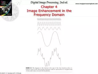
Chap 4 Image Enhancement in the Frequency Domain. Any periodic function can be expressed as the sum of sines and cosines of different frequencies, each multiplied by a different coefficient. We called this sum a Fourier series.

E N D
Any periodic function can be expressed as the sum of sines and cosines of different frequencies, each multiplied by a different coefficient. We called this sum a Fourier series. Even function that are not periodic can be expressed as the integral of sines and cosines multiplied by a weighting function. This formation is the Fourier transform. Background
A function f is periodic with period P greater than zero if Af(x + P) = Af(x), where A denotes amplitude. f(x) = sinx, P = 2π, frequency=1/ 2π, A=1. f(x) = Asinnx, P = 2π/n, frequency=n/ 2 π. n↑, frequency↑. Periodic Function
Fourier Series • Suppose f(x) is a function defined on the interval [-π,π]. The Fourier series expansion of f(x) is where an and bn are constants called the Fourier coefficients, and
Replace v by πx/L to obtain the Fourier series of the function ƒ(x) of period 2L Coefficients of Any Period T = 2L
Complex Fourier Series • Complex exponentials • According to Euler’s formula and so, Using these two equations we can find the complex exponential form of the trigonometric functions as
Continuous Spectra • Consider the following function: • Only a single pulse remains and the resulting function is no longer periodic. A function which is not periodic can be considered as a function with very large period.
Continuous Spectra These two integrals form the conclusion of Fourier’s integral theorem.
Alternative Forms • Note that there are a number of alternative forms for Fourier transform, such as • The third form is popular in the field of signal processing and communications systems.
Fourier transform F(u) of f(x) is defined as The inverse Fourier Transform is DFT for Discrete function f(x), x=0,1,..M-1 for u=0,1,..M-1 Inverse DFT 4.2 Fourier Transform in theFrequency Domain
Euler’s formula: Each term of the Fourier transform is composed of the sum of all values of the function f(x). M2summations and multiplications The values of f(x) are multiplied by sines and cosines of various frequencies. The domain (values of u) over which the values of F(u) range is appropriately called the frequency domain, because u determines the frequency of the components of the transform. Each of the M terms of F(u) is called a frequency component of the transform.
In general, the components of Fourier transform are complex quantities in the following form: F(u) = R(u) + jI(u) and can be written as F(u) = |F(u)|ej(u) The spectra is usually represented by the amplitude of a specific frequency Amplitude or spectrum of Fourier transform |F(u)| = (R2(u)+I2(u))1/2 Complex Spectra
Complex Spectra • These complex coefficients couples • Amplitude spectrum value • Magnitude of each of the harmonic components. • Phase spectrum value • The phase of each harmonic relative to the fundamental harmonic frequency ω0.
The frequency spectrum is centered at 0. To visual easily, we sometimes multiply f(x) by (-1)x before applying the transform.
2D-DFT of f(x, y) of size MN Inverse 2-D DFT 4.2.2 The Two-dimensional Discrete Fourier Transform (DFT)
Modulation in the space domain F[(-1)x+yf(x, y)]= F(u-M/2,v-N/2) Shift the origin of F(u,v) to frequency coordinates (M/2, N/2), the center of (u, v), u=0,…M-1, v=0,…N-1. frequency rectangle Average of f(x,y) For real f(x,y) F(u, v) = F*(-u, -v) |F(u, v)| = |F(-u, -v)| The spectrum of the Fourier transform is symmetric.
What is the “frequency” of an image? Since frequency is directly related rate of change, it is not difficult intuitively to associate frequencies with pattern of intensity variations in an image. The low frequencies correspond to the slowly varying components of an image. The higher frequencies begin to correspond to faster and faster gray level changes in the image. such as edges. F(0, 0): the average gray level of an image. 4.2.3 Filtering in the Frequency Domain
Multiply the input image by (-1)x+y to center the transform. Compute DFT F(u, v) Multiply F(u,v) by a filter function H(u,v) G(u,v) = F(u,v)H(u,v) Computer the inverse DFT of G(u,v) Obtain the real part of g(x,y) Multiply g(x,y) with (-1)x+y Filtering steps:
Notch filter: H(u,v) = 0 if (u,v) = (M/2, N/2), H(u,v) = 1 otherwise
Lowpass filter Highpass filter
The discrete convolution f(x,y)*h(x,y) f(x,y)*h(x,y) F(u,v)H(u,v) f(x,y)h(x,y) F(u,v)*H(u,v) 4.2.4 Filtering in spatial and frequency domains
Frequency-Domain Filtering: G(u,v) = H(u,v)F(u,v) Filter H(u,v) Ideal filter Butterworth filter Gaussian Filter 4.3 Smoothing Frequency-Domain Filters
H(u,v) = 1 if D(u,v) D0 = 0 if D(u,v) > D0 The center is at (u,v)=(M/2, N/2) D(u,v)=[(u-M/2)2 + (v-N/2)2]1/2 Cutoff frequency is D0 Power estimate: The percentage α of power enclosed in the circle is: 4.3.1 Ideal Low pass filter
The blurring in this image is a clear indication that most of the sharp detail information in the picture is contained in the 8% power removed by the filter. • The result of α =99.5 is quite close to the original, indicating little edge information is contained in the upper 0.5% of the spectrum power.
Butterworth lowpass filter (BLPF) of order n At the frequency as an half of the cutoff frequency D0, H(u, v)=0.5. 4.3.2 Butterworth Lowpass Filter
Gaussian filter Let =D0 When D(u, v)=D0 , H(u, v)=0.667 4.3.3 Gaussian Lowpass Filter
Highpass filtering: Hhp(u,v)=1-Hlp(u,v) Given a lowpass filter Hlp(u,v), find the spatial representation of the highpass filter Compute the inverse DFT of Hlp(u,v) Multiply the real part of the result with (-1)x+y 4.4 Sharpening Frequency-Domain Filter
H(u,v)=0 if D(u,v)D0 =1 if D(u,v)>D0 The center is at (u,v)=(M/2, N/2) D(u,v)=[(u-M/2)2+(v-N/2)2]1/2 Cutoff frequency is D0 4.4.1 Ideal Highpass Filter
Butterworth filter has no sharp cutoff At cutoff frequency D0: H(u, v)=0.5 4.4.2 Butterworth Highpass Filter