Download
1 / 43
520 likes | 561 Views
Image Enhancement in the Spatial Domain. Image Enhancement. The objective of Image Enhancement is to process image data so that the result is more suitable than the original image. Enhanced Image. Original Image. Enhancement Operator. Image Enhancement.

E N D
Image Enhancement The objective of Image Enhancement is to process image data so that the result is more suitable than the original image Enhanced Image Original Image Enhancement Operator
Image Enhancement Suppress or remove unwanted information. Example:
Image Enhancement Enhance features that are important to further processing.
Image Enhancement Image enhancement techniques can be applied to make human visual interpretation of images easier.
Image Enhancement Image Enhancement Spatial Domain Frequency Domain
Spatial Domain Enhancement The term spatial domain refers to the image plane itself, and approaches in this category are based on direct manipulation of pixels in an image
Spatial Domain Enhancement • Let f(x,y) be the original image and g(x,y) be the processed image Then where T is an operator over a certain neighborhood of the image centered at (x,y) Usually, we operate on a small rectangular region around (x,y)
Intensity Mapping • The simplest form of T is when the neighborhood is 1 x 1 pixel (single pixel) • In this case, g depends only on the gray level at (x,y) Intensity Mapping Output Gray level Input Gray level
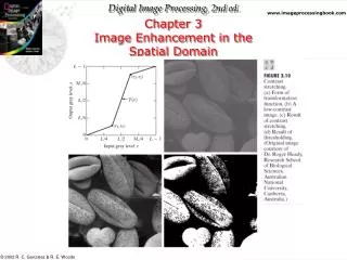
Example this technique is known as contrast stretching For example, if T(r) has the form shown in Fig. 3.2(a), the effect of this transformation would be to produce an image of higher contrast than the original by darkening the levels below m and brightening the levels above m in the original image.
Intensity mapping is used to : a)Increase Contrast b)Vary range of gray Levels • In the limiting case shown in Fig. 3.2(b), • T(r) produces a two-level (binary) image. A mapping of this form is called a thresholdingfunction
Intensity Mapping Fig (3.2) Because enhancement at any point in an image depends only on the gray level at that point, techniques in this category often are referred to as point processing
Mask processing or Filtering The general approach is to use a function of the values of f in a predefined neighborhood of (x, y) to determine the value of g at (x, y). One of the principal approaches in this formulation is based on the use of so-called masks (also referred to as filters, kernels, templates, or windows). Basically, a mask is a small (say, 3*3) 2-D array,
Some Basic Gray Level Transformations • As an introduction to gray-level transformations, consider Fig. 3.3, which shows three basic types of functions used frequently for image enhancement • linear (negative and identity transformations), • logarithmic (log and inverse-log transformations), • power-law (nth power and nth root transformations)
Some Basic Gray Level Transformations • A) Image Negative Example: L=256 The original image is a digital mammogram showing a small lesion This operation enhances details in dark regions
Some Basic Gray Level Transformations • B) Log Transformations this transformation maps a narrow range of low gray-level values in the input image into a wider range of output levels. The opposite is true of higher values of input levels. We would use a transformation of this type to expand the values of dark pixels in an image while compressing the higher-level values. The opposite is true of the inverse log transformation
Some Basic Gray Level Transformations Fourier Spectrum and Result of applying log transformation c=1
Some Basic Gray Level Transformations • C) Power Transformation • where c and ᵞ are positive constants
power-law curves with fractional values of ᵞ map a narrow range of dark input values into a wider range of output values, with the opposite being true for higher values of input levels A variety of devices used for image capture, printing, and display respond according to a power law.
Gamma Correction The process used to correct this power-law response phenomena is called gamma correction For example, cathode ray tube CRT devices have an intensity-to-voltage response that is a power function, with exponents varying from approximately 1.8 to 2.5.With reference to the curve for ᵞ =2.5
Gamma Correction we see that such display systems would tend to produce images that are darker than intended. Figure 3.7(a) shows a simple gray-scale linear wedge input into a CRT monitor. As expected, the output of the monitor appears darker than the input, as shown in Fig. 3.7(b). Gamma correction in this case is straightforward.
Gamma Correction • All we need to do is preprocess the input • image before inputting it into the monitor by performing the transformations : S = r1/2.5 = r0.4. • The result is shown in Fig. 3.7(c).When input into the same monitor, this gamma-corrected input produces an output that is close in appearance to the original image, as shown in Fig. 3.7(d)
Gamma Correction Fig. 3.7
Gamma Correction FIGURE 3.8 (a) Magnetic resonance (MR) image of a fractured human spine. (b)–(d) Results of applying the transformation in with c=1 and ᵞ=0.6, 0.4, and 0.3, respectively.
Gamma Correction Fig. 3.8
Gamma Correction Figure 3.9(a) shows the opposite problem of Fig. 3.8(a).The image to be enhanced now has a washed-out (باهت)appearance,indicating that a compression of graylevels is desirable.This can be accomplished with using values of ᵞgreater than 1.
Gamma Correction • The results of processing Fig. 3.9(a) with ᵞ=3.0, 4.0, and 5.0are shown in Figs. 3.9(b) through (d). Suitable results were obtained with gammavalues of 3.0 and 4.0, the latter having a slightly more appealingappearance becauseit has higher contrast. • The result obtained with g=5.0 has areas that aretoo dark, in which some detail is
Gamma Correction lost.The dark region to the left of the main roadin the upper left quadrant is an example of such an area.
Gamma Correction Fig. 3.9
Piecewise-Linear Transformation Functions • piecewise • linear functions are arbitrarily complex Contrast stretching
Low-contrast images can result from poor illumination, lack of dynamic range in the imaging sensor, or even wrong setting of a lens aperture during image acquisition. The idea behind contrast stretching is to increase the dynamic range of the gray levels in the image being processed.
Gray-level slicing Highlighting a specific range of gray levels in an image. Applications include enhancing features such as masses of water in satellite imagery and enhancing flaws in X-ray One approach to achieve this is to display a high value for all gray levels in the range of interest and a low value for all other gray levels.as in Fig. 3-11
The second approach, based on the transformation shown in Fig. 3.11(b), brightens the desired range of gray levels but preserves the background and gray-level tonalities (تناغم) in the image.
Contrast Stretching Fig. 3-11
Bit-plane slicing Instead of highlighting gray-level ranges,highlighting the contribution made tototal image appearance by specific bits might be desired. Suppose that eachpixel in an image is represented by 8 bits. Imagine that the image is composedof eight 1-bit planes, ranging from bit-plane 0 for the least significant bit to bitplane7 for the most significant bit. In terms of 8-bit bytes, plane 0 contains allthe lowest order bits in the bytes comprising the pixels in the image and plane7 contains all the high-order bits.
Note that thehigher-order bits (especially the top four) contain the majority of the visually significant data.The other bit planes contribute to more subtle details in the image.
Histogram • The Histogram of a digital image is a function : where rk is the kth gray level nkis the number of pixels having gray level rk
0 0 2 2 1 1 2 5 1 1 3 4 2 2 3 4 Histogram • Example:
Normalized Histogram • Normally, we normalize h(rk) by • So, we have • p(rk) can be sought of as the probability of a pixel to have a certain value rk
0 0 2 2 1 1 2 5 1 1 3 4 2 2 3 4 Normalized Histogram • Example: n=16
Histogram Note: Images with uniformlyDistributed histograms have higher Contrast and highdynamic range