Download
1 / 34
440 likes | 735 Views
Chap. 3: Image Enhancement in the Spatial Domain. Spring 2006, Jen-Chang Liu CSIE, NCNU. Announcement. Where to find MATLAB ? It ’ s not free … A book contains the student ’ s edition of MATLAB NCNU CC support 50 on-line version in the computer rooms (307, 308, 208, 413). Image Enhancement.

E N D
Chap. 3: Image Enhancement in the Spatial Domain Spring 2006, Jen-Chang Liu CSIE, NCNU
Announcement • Where to find MATLAB ? • It’s not free… • A book contains the student’s edition of MATLAB • NCNU CC support 50 on-line version in the computer rooms (307, 308, 208, 413)
Image Enhancement • Goal: process an image so that the result is more suitable than the original image for a specific application • Visual interpretation • Problem oriented
Two categories • There is no general theory of image enhancement • Spatial domain • Direct manipulation of pixels • Point processing • Neighborhood processing • Frequency domain • Modify the Fourier transform of an image
Outline: spatial domain operations • Background • Gray level transformations • Arithmetic/logic operations
f(x,y) g(x,y) T Background • Spatial domain processing • g(x,y)=T[ f(x,y) ] • f(x,y): input image • g(x,y): output image • T: operator • Defined over some neighborhood of (x,y)
Background (cont.) * T applies to each pixel in the input image * T operates over neighborhood of (x,y)
thresholding Point processing • 1x1 neighborhood • Gray level transformation, or point processing • s = T(r) contrast stretching
Neighborhood processing • A larger predefined neighborhood • Ex. 3x3 neighborhood • mask, filters, kernels, templates, windows • Mask processing or filtering
Some Basic Gray Level Transformations • Image negatives (complement) • Log transformation • Power-law transform • Piece-wise linear transform • Gray level slicing • Bit plane slicing
Some gray level transformations • Lookup table • Functional form
Image negatives • Photographic negative 負片 • Suitable for images with dominant black areas Original mammogram(乳房X光片)
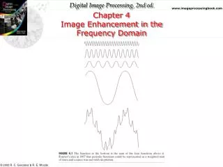
Log transformations • s = c log(1+r) • Compress the dynamic range of images with large variation in pixel values
Example: Log transformations • log(fft2(I)) : log of Fourier transform log 2d Fourier transform 頻譜圖
Power-law transformations • s=cr • >1 • <1 • : gamma • display, printers, scanners follow power-law • Gamma correction
=1/2.5 =2.5 Example: Gamma correction 顯示器偏差 原始影像 • CRT: intensity-to-voltage response follow a power-law. 1.8<<2.5 =2.5
<1 Power-law: • Expand dark gray levels =0.6 =0.4 =0.3
Power-law: >1 • Expand light gray levels =3 =4 =5
Piece-wise linear transformations control point • Advantage: the piecewise function can be arbitrarily complex
Contrast stretching How to automatically adjust the gray levels?
Gray-level slicing 切片 • Highlighting a specific range of gray levels
1 0 0 1 0 1 0 0 Ex. 15010 Bit-plane slicing * Highlight specific bits bit-planes of an image (gray level 0~255)
For image compression 6 7 5 3 4 0 1 2
Arithmetic/logic operations • Logic operations • Image subtraction • Image averaging
Logic operations • Logic operations: pixel-wise AND, OR, NOT • The pixel gray level values are taken as string of binary numbers • Use the binary mask to take out the region of interest(ROI) from an image Ex. 193 => 11000001
Logic operations: example A B A and B AND A or B OR
Image subtraction f:original(8 bits) h:4 sig. bits • Difference image g(x,y)=f(x,y)-h(x,y) scaling difference image
Image subtraction: scaling the difference image • g(x,y)=f(x,y)-h(x,y) • f and h are 8-bit => g(x,y) [-255, 255] • (1)+255 (2) divide by 2 • The result won’t cover [0,255] • (1)-min(g) (2) *255/max(g) Be careful of the dynamic range after the image is processed.
Image subtraction example: mask mode radiography • Inject contrast medium into bloodstream original (head) difference image 注射碘液 拍攝影像 與原影像 相減
Image averaging • Noisy image g(x,y)=f(x,y)+η(x,y) • Suppose η(x,y) is uncorrelated and has zero mean original noise Clear image Noisy image
Image averaging: noise reduction • Averaging over K noisy images gi(x,y) 期望值接近原圖
original Gaussian noise averaging K=8 averaging K=16 averaging K=64 averaging K=128