Download
1 / 38
380 likes | 501 Views
Explore advanced techniques in sequence alignment, focusing on methods that utilize linear space complexity (O(m)) instead of the typical O(mn). This approach implements Hirschberg's algorithm and divide-and-conquer strategies to optimize space usage while ensuring accurate alignment. Additionally, it discusses k-difference global alignment and inexact matching, emphasizing computational efficiency through bounded differences and dynamic programming. Discover how to tackle alignment challenges while conserving resources effectively.

E N D
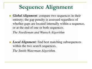
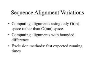
Sequence Alignment Variations • Computing alignments using only O(m) space rather than O(mn) space. • Computing alignments with bounded difference • Exclusion methods: fast expected running times
1. Linear Space • Hirschberg [1977] • Suppose we only need the maximum similarity value of S and T without an alignment or transcript • How can we conserve space? • Only save row i-1 when computing row i in the table
0 1 2 3 4 n n-1 Illustration 0 1 2 3 4 5 6 7 … m . . .
Linear space and an alignment • Assume S has length 2n • Divide and conquer approach • Compute value of optimal alignment of S[1..n] with all prefixes of T • Store row n only at end along with pointer values of row n • Compute value of optimal alignment of Sr[1..n] with all prefixes of Tr • Store only values in row n • Find k such that • V(S[1..n],T[1..k]) + V(Sr[1..n],Tr[1..m-k]) • is maximized over 0 <= k <=m
V(S[1..6], T[1..0]) V(Sr[1..6], Tr[1..18]) Illustration k=0 0 1 2 3 4 5 6 7 8 9 0 1 2 3 4 5 6 7 8 - 0 1 2 3 4 5 6 m-k=18 6 5 4 3 2 1 0 - 8 7 6 5 4 3 2 1 0 9 8 7 6 5 4 3 2 1 0
V(S[1..6], T[1..1]) V(Sr[1..6], Tr[1..17]) Illustration k=1 0 1 2 3 4 5 6 7 8 9 0 1 2 3 4 5 6 7 8 - 0 1 2 3 4 5 6 m-k=17 6 5 4 3 2 1 0 - 8 7 6 5 4 3 2 1 0 9 8 7 6 5 4 3 2 1 0
V(S[1..6], T[1..2]) V(Sr[1..6], Tr[1..16]) Illustration k=2 0 1 2 3 4 5 6 7 8 9 0 1 2 3 4 5 6 7 8 - 0 1 2 3 4 5 6 m-k=16 6 5 4 3 2 1 0 - 8 7 6 5 4 3 2 1 0 9 8 7 6 5 4 3 2 1 0
V(S[1..6], T[1..9]) V(Sr[1..6], Tr[1..9]) Illustration k=9 0 1 2 3 4 5 6 7 8 9 0 1 2 3 4 5 6 7 8 - 0 1 2 3 4 5 6 m-k=9 6 5 4 3 2 1 0 - 8 7 6 5 4 3 2 1 0 9 8 7 6 5 4 3 2 1 0
V(S[1..6], T[1..18]) V(Sr[1..6], Tr[1..0]) Illustration k=18 0 1 2 3 4 5 6 7 8 9 0 1 2 3 4 5 6 7 8 - 0 1 2 3 4 5 6 m-k=0 6 5 4 3 2 1 0 - 8 7 6 5 4 3 2 1 0 9 8 7 6 5 4 3 2 1 0
Illustration 0 1 2 3 4 5 6 7 8 9 0 1 2 3 4 5 6 7 8 - 0 1 2 3 4 5 6 6 5 4 3 2 1 0 - 8 7 6 5 4 3 2 1 0 9 8 7 6 5 4 3 2 1 0
Recursive Step • Let k* be the k that maximizes • V(S[1..n],T[1..k]) + V(Sr[1..n],Tr[1..m-k]) • Record all steps on row n including the one from n-1 and the one to n+1 • Recurse on the two subproblems • S[1..n-1] with T[1..j] where j <= k* • Sr[1..n] with Tr[1..q] where q <= m-k*
Illustration 0 1 2 3 4 5 6 7 8 9 0 1 2 3 4 5 6 7 8 - 0 1 2 3 4 5 6 6 5 4 3 2 1 0 - 8 7 6 5 4 3 2 1 0 9 8 7 6 5 4 3 2 1 0
Time Required • cmn time to get this answer so far • Two subproblems have at most half the total size of this problem • At most the same cmn time to get the rest of the solution • cmn/2 + cmn/4 + cmn/8 + cmn/16 + … <= cmn/2 • Final result • Linear space with only twice as much time
Extending to local alignment • What are the problems? • Don’t know what substrings of S and T to align, so we won’t know midpoints • Solution • Find end point by computing only values and storing max value (and location) along the way • Find start point by computing a “reversed” dynamic program using the reverse strings starting at i in S and j in T • Once end points are fixed, just like global alignment
2. Bounded Difference • Suppose the number of differences between S and T is bounded • Typically focus on (unweighted) edit distance • Can we speed things up? • Motivation: • pages 260-263
Problem Definition 1 • k-difference global alignment • Input • Strings S and T • Task • Find best global alignment of S and T containing at most k mismatches and spaces or say that no such alignment exists
Problem Definition 2 • k-difference inexact matching • Input • Strings P and T • Task • Find all ways, if any, to match P in T using at most k character substitutions, insertions, and deletions, or report that no such matches exist. • End spaces in T but not P are free
Earlier Problem Definition • k-mismatch problem • Input • Strings P and T • Task • Find all ways, if any, to match P in T using at most k character substitutions, insertions, and deletions, or report that no such matches exist. • No internal spaces
Example • Difference between k-mismatch problem and the k-difference problem • Inputs • P = abcdefghi • T = abcdeefghi • Minimum # of mismatches is 4 • Minimum # of differences is 1 with 1 space in P after the e
Solution for k-difference global alignment • Compute edit distance of S and T but only fill in an O(km)-size portion of the table • Work only with diagonals that are within k of the main diagonal • If result in D(n,m) is <= k, then there is an optimal alignment • If result in D(n,m) is >k, then the optimal alignment has value > k (though possibly less than D(n,m)
Illustration 0 1 2 3 4 5 6 7 8 9 0 1 2 3 0 1 2 3 4 5 6 7 8 9 0 1 2 3 k=4
Unknown k* • Suppose we don’t know the optimal k* a priori • Use doubling trick to guess k* • Start with k=1 • Then k=2 • Then k=4 • Then k=8 • … • Final work will be O(k*m)
k-difference inexact matching • Solution method • O(km) time and space solution for the problem • Can be reduced to O(m+n) space if we only want the end position in T of the match • Hybrid dynamic programming • Use suffix trees with longest common extension together with dynamic programming to solve this problem • Note, the first row of table will be 0 to reflect end spaces in T are free
Definitions • Diagonals are numbered • 1 to m above main diagonal • -1 to -n below the main diagonal • A d-path in the dynamic programming table is a path that starts in row 0 and specifies a total of d mismatches and spaces • A d-path is farthest reaching in diagonali if • it is a d-path that ends in diagonal i and • its ending column c is >= the ending column of any other d-path that ends in diagonal i
Illustration 12 3 4 5 6 7 8 9 0 1 2 3 0 -1 -2 -3 -4 -5 -6 -7 -8 -9
Approach • To compute farthest-reaching d-path on diagonal i • Take farthest-reaching (d-1)-path on diagonal i+1 • Move down one square, and then do a longest common extension from that point • Take farthest-reaching (d-1)-path on diagonal i-1 • Move right one square, and then do a longest common extension from that point • Take farthest-reaching (d-1)-path on diagonal i • Move diagonally one square, and then do a longest common extension from that point
Diagonal i+1 (d-1)-path 1 234 5 6 7 8 9 0 1 2 3 0 -1 -2 -3 -4 -5 -6 -7 -8 -9 Finding longest 1-path on diagonal 3 using longest 0-paths on diagonals 2, 3, and 4 as a starting point.
Diagonal i-1 (d-1)-path 1 234 5 6 7 8 9 0 1 2 3 0 -1 -2 -3 -4 -5 -6 -7 -8 -9 Finding longest 1-path on diagonal 3 using longest 0-paths on diagonals 2, 3, and 4 as a starting point.
Diagonal i (d-1)-path 1 234 5 6 7 8 9 0 1 2 3 0 -1 -2 -3 -4 -5 -6 -7 -8 -9 Finding longest 1-path on diagonal 3 using longest 0-paths on diagonals 2, 3, and 4 as a starting point.
High level outline • d = 0; • For i = 0 to m do • find longest common extension of P(1) and T(i) • This is the 0-path on diagonal i • For d = 1 to k do • For i = -n to m do • using farthest reaching (d-1) paths on diagonals i-1, i, and i+1, find farthest reaching d-path on diagonal i • Any path that reaches row n defines an inexact match of P in T that contains at most k differences
3. Exclusion Methods • Previous methods still have running time Q(km) • Can we get to expected times of O(m) or even smaller? • Note, we are not asking for worst-case times this small. • For example, Boyer-Moore has sublinear time for the exact matching problem
Partition Idea • Partition T or P into consecutive regions of a given length r • Search/Filter Phase • Using various exact matching methods, search using these partition values to filter out possible locations of P in T • Check phase • For each surviving location, use an approximate matching technique to verify an approximate occurrence of P
BYP Choices • Baeza-Yates and Perleberg • O(m) expected running time for modest error rates • Let r = floor(n/(k+1)) • Partition P into consecutive length-r intervals • last interval may have length less than r • Key property • There are at least k+1 intervals of P that have full length r • If P matches a substring T’ of T with at most k differences, then T’ must contain one interval of length r that matches one of the k+1 intervals of P exactly.
BYP Algorithm • Let P’ be the set of k+1 substrings of P taken from the first k+1 regions of P’s partition • Build a keyword tree for P’ • Using Aho-Corasick, find I, the set of all starting locations in T where any pattern in P occurs exactly • For each i in I, use an approximate matching algorithm (probably based on dynamic programming) to locate end points of all approximate occurrences of P in substring T[i-n-k..i+n+k]
Running Time Analysis • Search phase: O(n+m) time and O(n) space • We could use suffix trees or suffix trees and matching statistics as well for similar performance • We could use Boyer-Moore set matching techniques described in Section 7.16 to speed this up even more • Check Phase • Dynamic programming takes O(n2) time per location checked • Previous results can be used for O(kn) time per location checked
Expected running time • Need to get expected size of number of locations to be checked • Probability model • Each character of T is drawn uniformly at random from the alphabet of size q • An upper bound on the expected number of occurrences of a region p from P’ in T is m(k+1)/qr • T has roughly m substrings of length r • Each substring matches an individual p with probability 1/qr
Expected running time • Expected time of checking: [m(k+1)/qr] n2 • (number of occurrences) x (time per occurrence) • Need to determine what values of k make this cost <= a constant times m • Some mathematical manipulation leads to BYP is O(m) as long as k = O(n/log n) • That is, error rate is less than 1 every log n characters
Extensions • See the book, pages 273-279, for some extensions to these ideas • The expected work can be made sublinear