Sequence Alignment

1. Sequence Alignment

2. Outline • Global Alignment • Scoring Matrices • Local Alignment • Alignment with Affine Gap Penalties

3. From LCS to Alignment: Change Scoring • The Longest Common Subsequence (LCS) problem—the simplest form of sequence alignment – allows only insertions and deletions (no mismatches). • In the LCS Problem, we scored 1 for matches and 0 for indels • Consider penalizing indels and mismatches with negative scores • Simplest scoring schema: +1 : match premium -μ : mismatch penalty -σ : indel penalty

4. Simple Scoring • When mismatches are penalized by –μ, indels are penalized by –σ, and matches are rewarded with +1, the resulting score is: #matches – μ(#mismatches) – σ (#indels)

5. The Global Alignment Problem Find the best alignment between two strings under a given scoring schema Input : Strings v and w and a scoring schema Output : Alignment of maximum score → = -б = 1 if match = -µ if mismatch si-1,j-1 +1 if vi = wj si,j = max s i-1,j-1 -µ if vi ≠ wj s i-1,j - σ s i,j-1 - σ m : mismatch penalty σ : indel penalty {

6. Scoring Matrices To generalize scoring, consider a (4+1) x(4+1) scoring matrixδ. In the case of an amino acid sequence alignment, the scoring matrix would be a (20+1)x(20+1) size. The addition of 1 is to include the score for comparison of a gap character “-”. This will simplify the algorithm as follows: si-1,j-1 + δ(vi, wj) si,j = max s i-1,j + δ(vi, -) s i,j-1 + δ(-, wj) {

7. Measuring Similarity • Measuring the extent of similarity between two sequences • Based on percent sequence identity • Based on conservation

8. Percent Sequence Identity • The extent to which two nucleotide or amino acid sequences are invariant A C C T G A G – A G A C G T G – G C A G mismatch indel 70% identical

9. Making a Scoring Matrix • Scoring matrices are created based on biological evidence. • Alignments can be thought of as two sequences that differ due to mutations. • Some of these mutations have little effect on the protein’s function, therefore some penalties, δ(vi , wj), will be less harsh than others.

10. AKRANR KAAANK -1 + (-1) + (-2) + 5 + 7 + 3 = 11 Scoring Matrix: Example • Notice that although R and K are different amino acids, they have a positive score. • Why? They are both positively charged amino acids will not greatly change function of protein.

11. Scoring matrices • Amino acid substitution matrices • PAM • BLOSUM • DNA substitution matrices • DNA is less conserved than protein sequences • Less effective to compare coding regions at nucleotide level

12. PAM • Point Accepted Mutation (Dayhoff et al.) • 1 PAM = PAM1 = 1% average change of all amino acid positions • After 100 PAMs of evolution, not every residue will have changed • some residues may have mutated several times • some residues may have returned to their original state • some residues may not changed at all

13. PAMX • PAMx = PAM1x • PAM250 = PAM1250 • PAM250 is a widely used scoring matrix: Ala Arg Asn Asp Cys Gln Glu Gly His Ile Leu Lys ... A R N D C Q E G H I L K ... Ala A 13 6 9 9 5 8 9 12 6 8 6 7 ... Arg R 3 17 4 3 2 5 3 2 6 3 2 9 Asn N 4 4 6 7 2 5 6 4 6 3 2 5 Asp D 5 4 8 11 1 7 10 5 6 3 2 5 Cys C 2 1 1 1 52 1 1 2 2 2 1 1 Gln Q 3 5 5 6 1 10 7 3 7 2 3 5 ... Trp W 0 2 0 0 0 0 0 0 1 0 1 0 Tyr Y 1 1 2 1 3 1 1 1 3 2 2 1 Val V 7 4 4 4 4 4 4 4 5 4 15 10

14. PAM250 log odds scoring matrix

15. Why do we go from a mutation probability matrix to a log odds matrix? • We want a scoring matrix so that when we do a pairwise • alignment (or a BLAST search) we know what score to • assign to two aligned amino acid residues. • Logarithms are easier to use for a scoring system. They • allow us to sum the scores of aligned residues (rather • than having to multiply them).

16. How do we go from a mutation probability matrix to a log odds matrix? • The cells in a log odds matrix consist of an “odds ratio”: • the probability that an alignment is authentic • the probability that the alignment was random • The score S for an alignment of residues a,b is given by: • S(a,b) = 10 log10 ( Mab / pb ) • As an example, for tryptophan, • S( W, W ) = 10 log10 ( 0.55 / 0.01 ) = 17.4

17. What do the numbers mean in a log odds matrix? S( W, W ) = 10 log10 ( 0.55 / 0.010 ) = 17.4 A score of +17 for tryptophan means that this alignment is 50 times more likely than a chance alignment of two tryptophan residues. S(W, W) = 17 Probability of replacement ( Mab / pb ) = x Then 17 = 10 log10 x 1.7 = log10 x 101.7 = x = 50

18. What do the numbers mean in a log odds matrix? A score of +2 indicates that the amino acid replacement occurs 1.6 times as frequently as expected by chance. A score of 0 is neutral. A score of –10 indicates that the correspondence of two amino acids in an alignment that accurately represents homology (evolutionary descent) is one tenth as frequent as the chance alignment of these amino acids.

19. PAM10 log odds scoring matrix

20. BLOSUM Outline • Idea: use aligned ungapped regions of protein families.These are assumed to have a common ancestor. Similar ideas but better statistics and modeling. • Procedure: • Cluster together sequences in a family whenever more than L% identical residues are shared, for BLOSUM-L. • Count number of substitutions across different clusters (in the same family). • Estimate frequencies using the counts. • Practice: BlOSUM-50 and BLOSOM62 are wildly used. Considered the state of the art nowadays.

21. BLOSUM Matrices BLOSUM matrices are based on local alignments. BLOSUM stands for blocks substitution matrix. BLOSUM62 is a matrix calculated from comparisons of sequences with less than 62% identical sites.

22. BLOSUM Matrices 100 collapse 62 Percent amino acid identity 30 BLOSUM62

23. BLOSUM Matrices 100 100 100 collapse collapse 62 62 62 collapse Percent amino acid identity 30 30 30 BLOSUM80 BLOSUM62 BLOSUM30

24. BLOSUM Matrices All BLOSUM matrices are based on observed alignments; they are not extrapolated from comparisons of closely related proteins. The BLOCKS database contains thousands of groups of multiple sequence alignments. BLOSUM62 is the default matrix in BLAST 2.0. Though it is tailored for comparisons of moderately distant proteins, it performs well in detecting closer relationships. A search for distant relatives may be more sensitive with a different matrix.

25. Blosum62 scoring matrix

26. Rat versus mouse RBP Rat versus bacterial lipocalin

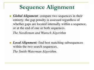
27. Local vs. Global Alignment • The Global Alignment Problem tries to find the longest path between vertices (0,0) and (n,m) in the edit graph. • The Local Alignment Problem tries to find the longest path among paths between arbitrary vertices (i,j) and (i’, j’) in the edit graph.

28. Local vs. Global Alignment • The Global Alignment Problem tries to find the longest path between vertices (0,0) and (n,m) in the edit graph. • The Local Alignment Problem tries to find the longest path among paths between arbitrary vertices (i,j) and (i’, j’) in the edit graph. • In the edit graph with negatively-scored edges, Local Alignmet may score higher than Global Alignment

29. Local vs. Global Alignment (cont’d) • Global Alignment • Local Alignment—better alignment to find conserved segment --T—-CC-C-AGT—-TATGT-CAGGGGACACG—A-GCATGCAGA-GAC | || | || | | | ||| || | | | | |||| | AATTGCCGCC-GTCGT-T-TTCAG----CA-GTTATG—T-CAGAT--C tccCAGTTATGTCAGgggacacgagcatgcagagac |||||||||||| aattgccgccgtcgttttcagCAGTTATGTCAGatc

30. Compute a “mini” Global Alignment to get Local Local Alignment: Example Local alignment Global alignment

31. Local Alignments: Why? • Two genes in different species may be similar over short conserved regions and dissimilar over remaining regions. • Example: • Homeobox genes have a short region called the homeodomain that is highly conserved between species. • A global alignment would not find the homeodomain because it would try to align the ENTIRE sequence

32. The Local Alignment Problem • Goal: Find the best local alignment between two strings • Input : Strings v, w and scoring matrix δ • Output : Alignment of substrings of v and w whose alignment score is maximum among all possible alignment of all possible substrings

33. The Problem with this Problem • Long run time O(n4): - In the grid of size n x n there are ~n2 vertices (i,j) that may serve as a source. - For each such vertex computing alignments from (i,j) to (i’,j’) takes O(n2) time. • This can be remedied by giving free rides

34. Compute a “mini” Global Alignment to get Local Local Alignment: Example Local alignment Global alignment

35. Local Alignment: Example

36. Local Alignment: Example

37. Local Alignment: Example

38. Local Alignment: Example

39. Local Alignment: Example

40. Local Alignment: Running Time • Long run time O(n4): - In the grid of size n x n there are ~n2 vertices (i,j) that may serve as a source. - For each such vertex computing alignments from (i,j) to (i’,j’) takes O(n2) time. • This can be remedied by giving free rides

41. Local Alignment: Free Rides Yeah, a free ride! Vertex (0,0) The dashed edges represent the free rides from (0,0) to every other node.

42. Notice there is only this change from the original recurrence of a Global Alignment The Local Alignment Recurrence • The largest value of si,j over the whole edit graph is the score of the best local alignment. • The recurrence: 0 si,j = max si-1,j-1 + δ(vi, wj) s i-1,j + δ(vi, -) s i,j-1 + δ(-, wj) {

43. Power of ZERO: there is only this change from the original recurrence of a Global Alignment - since there is only one “free ride” edge entering into every vertex The Local Alignment Recurrence • The largest value of si,j over the whole edit graph is the score of the best local alignment. • The recurrence: 0 si,j = max si-1,j-1 + δ(vi, wj) s i-1,j + δ(vi, -) s i,j-1 + δ(-, wj) {

44. Scoring Indels: Naive Approach • A fixed penalty σis given to every indel: • -σ for 1 indel, • -2σ for 2 consecutive indels • -3σ for 3 consecutive indels, etc. Can be too severe penalty for a series of 100 consecutive indels

45. This is more likely. This is less likely. Affine Gap Penalties • In nature, a series of k indels often come as a single event rather than a series of k single nucleotide events: ATA__GC ATATTGC ATAG_GC AT_GTGC Normal scoring would give the same score for both alignments

46. Accounting for Gaps • Gaps- contiguous sequence of spaces in one of the rows • Score for a gap of length x is: -(ρ +σx) where ρ >0 is the penalty for introducing a gap: gap opening penalty ρ will be large relative to σ: gap extension penalty because you do not want to add too much of a penalty for extending the gap.

47. Affine Gap Penalties • Gap penalties: • -ρ-σ when there is 1 indel • -ρ-2σ when there are 2 indels • -ρ-3σ when there are 3 indels, etc. • -ρ- x·σ (-gap opening - x gap extensions) • Somehow reduced penalties (as compared to naïve scoring) are given to runs of horizontal and vertical edges

48. Affine Gap Penalties and Edit Graph To reflect affine gap penalties we have to add “long” horizontal and vertical edges to the edit graph. Each such edge of length x should have weight - - x *

49. Adding “Affine Penalty” Edges to the Edit Graph There are many such edges! Adding them to the graph increases the running time of the alignment algorithm by a factor of n (where n is the number of vertices) So the complexity increases from O(n2) to O(n3)

50. Manhattan in 3 Layers ρ δ δ σ δ ρ δ δ σ