Download
1 / 26
260 likes | 392 Views
“The past, the present and the future of global weather and climate modelling” Royal Meteorological Society meeting, University of Reading, 25 April 2007. Weather and climate modelling expands to cover the globe Tony Slingo, ESSC University of Reading. Scope: from the 1950s to the 1990s

E N D
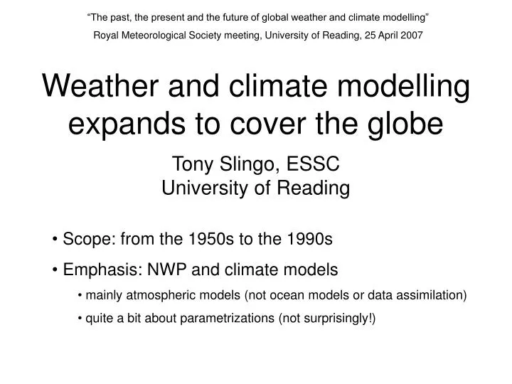
“The past, the present and the future of global weather and climate modelling” Royal Meteorological Society meeting, University of Reading, 25 April 2007 Weather and climate modelling expands to cover the globeTony Slingo, ESSCUniversity of Reading • Scope: from the 1950s to the 1990s • Emphasis: NWP and climate models • mainly atmospheric models (not ocean models or data assimilation) • quite a bit about parametrizations (not surprisingly!)
Early developments in the USA • 1950: Charney, Fjortoft and von Neumann • 1956: Phillips (first general circulation experiment) • The start of NWP and climate modelling • 1954: Joint Numerical Weather Prediction Unit • 1958: National Meteorological Center (NMC) • 1974: NMC ran the first global grid-point model • Geophysical Fluid Dynamics Laboratory (GFDL) • originally (1955) a section of the US Weather Bureau • led by Smagorinsky, with Manabe, Miyakoda, Bryan, … • 1963: 9 level primitive equation grid-point model • many firsts (hydrological cycle, coupled ocean-atmosphere, CO2) • University of California Los Angeles (UCLA) • grid-point model (Mintz/Arakawa) • Goddard Institute for Space Studies (GISS), GSFC and others • National Center for Atmospheric Research (NCAR) • grid-point model (Kasahara/Washington)
Early developments outside the USA • Several countries developed NWP and climate models • e.g. Sweden (1954), UK, France, Germany, Australia, Canada • more on the UK Met Office in a moment • First spectral model developed by Bourke (1972, 1974) • was exported to GFDL, where it replaced the grid-point model, and to NCAR, where it replaced the Kasahara/Washington model and became the Community Climate Model (CCM) • ECMWF was founded in 1975 • first model was global, grid-point (August 1979) • replaced by a spectral model in 1983 • exported to create the climate model at the Max Planck Institute for Meteorology, in Hamburg
Some other key international developments • 1957-58: IGY • International Geophysical Year • 1967: GARP • Global Atmospheric Research Programme • 1974: GATE • GARP Atlantic Tropical Experiment • the first large-scale tropical experiment • 1978-1979: FGGE • First GARP Global Experiment • global weather observations for an entire year • coincided with the launch of Tiros-N
NWP and climate modelling in the Met Office • NWP • 1959 (Ferranti Mercury): experimental 2-level limited area model • 1965 (KDF 9): 3-level quasi-geostrophic model operational • 1972 (IBM 360/195): 10-level primitive equation model (Bushby) • Northern Hemisphere, and embedded European “rectangle” • 1982 (CDC Cyber 205): 15-level, 150km, 144h global forecasts • Climate • 5-level model (Corby, Gilchrist and Newson, 1975) • 1972: 11-layer model, used as a tropical model for GATE by Peter Rowntree’s group • stratospheric model for the Comesa project • 1990: Hadley Centre for climate prediction and research • Unified Forecast/Climate Model • 1991 (Cray Y-MP): first version had 19 levels • 2002: New Dynamics • All of the above were/are grid-point models
Phillips (1956) “Certain of the assumptions in this particular numerical experiment can be eliminated in a rather straightforward manner, e.g. the geostrophic assumption and the simplified geometry. However, a further refinement of the model will soon run into the more difficult physical problems of small-scale turbulence and convection, the release of latent heat, and the dependence of radiation on temperature, moisture and cloud. Progress in the past in developing an adequate theory of the general circulation has had as its main obstacle the difficulty of solving the non-linear hydrodynamical equations. High-speed computing machines have to some extent eliminated this problem, and further progress in understanding the large-scale behaviour of the atmosphere should come to depend more and more on a fuller understanding of the physical processes mentioned above.”
Parametrization highlights • Convection • early models: simple convective adjustment • more advanced: mass-flux convection schemes • Arakawa and Schubert (1974) • Rowntree scheme: Lyne and Rowntree (1976) , Gregory and Rowntree (1990). Modified to include saturated downdraughts, convective momentum transfer • Betts and Miller (1986); convective adjustment scheme, ECMWF • Tiedtke (1989), ECMWF
Representation of orography The upper figure shows the surface orography over North America at a resolution of 300km, as in a low resolution climate model. The lower figure shows the same field at a resolution of 60km, as in a weather forecasting model.
Parametrization highlights • Orographic gravity wave drag • As the horizontal resolution of climate models improved, by the 1980s some models showed evidence of anomalously strong westerly winds at mid-latitudes • This was particularly noticeable in the Met Office 11-layer model and was known as the “westerly problem” • The problem was solved by Palmer, Shutts and Swinbank (1986), who developed a parametrization for the drag produced by gravity waves excited by unresolved orography • A similar parametrization was developed by McFarlane (1986) and used in the Canadian climate model
Parametrization highlights • Radiation • early models: prescribed from climatological calculations • more advanced: interactive radiation, clouds • Manabe and Strickler (1964) • 11-layer model (Walker 1977) • Lacis and Hansen (1974), which anticipated; • even more advanced: full scattering codes • Edwards and Slingo (1996), used in Unified Model • Mlawer et al. (1997), used in ECMWF model
Parametrizations and model resolution • Many of the parametrizations used in GCMs fall within the ambit of Phillips’ comments on the non-linear hydrodynamical equations • Radiation does not, but convection, boundary layer and wave drag processes do • For many of these processes, we have made little progress in understanding how to parametrize them, or even whether they can be parametrized at all • This suggests that we need to increase the resolution of GCMs substantially, either to resolve these motions explicitly or at least to give parametrizations a chance to work properly on scales that can be parametrized • Have climate modellers done this?
Progression of Met Office climate models from the original 11-layer model onwards
Why haven’t climate modellers increased the resolution of their models? • Because there have been other priorities: • standard runs of the 11-layer model on the IBM 360/195 were 50 days in length • but climate integrations (e.g. for global warming predictions) need complex models run on decadal to century timescales • so, all of the extra computing power has had to be directed towards longer integrations of more complex models, with ensembles to investigate different scenarios and to provide better signal to noise • In contrast, every time that more computing resources have become available, the resolution of NWP models has been increased • because high resolution is needed to assimilate the initial data properly and to provide regional detail in the forecasts • and of course weather forecasts are run for days, not years, and the models do not need to be quite so complicated
1/120 Complexity Computing Resources Resolution Duration and/or Ensemble size Resolution, complexity, duration/ensemble size
ConclusionIt is time to start running climate models at much higher resolution, not for all applications of course, but at least to try to make progress with the parametrization problem and to meet the challenge articulated by Phillips in 1956
Sources of information Don’t bother to copy all this down, go to http://www.nerc-essc.ac.uk/~as/ • Randall, D.A. (Ed.) 2000. General circulation model development. Academic Press • Washington, W.M. and Parkinson, C.L., 2005. An introduction to three dimensional climate modeling. University Science Books • Trenberth, K.E.,1995. Climate system modeling. Cambridge University Press • Web pages: • http://wwwt.ncep.noaa.gov/nwp50/ (meeting on 50th anniversary of NWP) • http://www.aip.org/history/sloan/gcm/intro.html (history of GCM modelling) • http://www.metoffice.gov.uk/research/nwp/publications/nwp_gazette/sep02/history_nwp.html (Met Office website) • http://celebrating200years.noaa.gov/historymakers/Smagorinsky/welcome.html (general website; this one about Joseph Smagorinsky) • http://www.bom.gov.au/bmrc/basic/wksp16/papers/papers.shtml (BMRC Workshop November 2004; several excellent talks) • http://www.ecmwf.int/newsevents/training/ (ECMWF website)