Download
1 / 25
250 likes | 389 Views
Comparison of fluxes with models Nazim Bharmal ESSC, University of Reading. ESSC 19 th July 2007. Study of divergence across atmosphere using data from AMF(s) and GERB. Partner to data are the model fluxes, here using the Edwards-Slingo code: Pristine-sky conditions (no aerosol, no cloud).

E N D
Comparison of fluxes with modelsNazim BharmalESSC, University of Reading ESSC 19th July 2007
Study of divergence across atmosphere using data from AMF(s) and GERB. • Partner to data are the model fluxes, here using the Edwards-Slingo code: • Pristine-sky conditions (no aerosol, no cloud). • Clear sky (with aerosol, no cloud). • All sky (with aerosol and cloud).
LW data and modelling • LW divergence from 3 components • DLR, downwelling LW radiation at the surface • OLR, outgoing LW radiation at TOA • GLR, ground-leaving LW radiation at the surface • (no incoming LW radiation c.f. shortwave) • This talk discusses the modelling of these 3 components and comparisons to data. • Discuss clear-sky cases only (no clouds)
DLR measurements • Three components drive clear-sky DLR
DLR modelling • DLR from Prata formula and ES (pristine sky)
Prata formula analysis • Analyse Prata formula at • higher temporal resolution
ES correlation • Correlation of DLR with PWV is significant.
ES correlation • Correlation of DLR with AERONET • derived AOT is also significant.
ES with aerosol ‘correction’ • Account for aerosol, leads • to clear-sky estimate
ES with aerosol ‘correction’ • Aerosol ‘correction’ makes distributions tighter as would be expected.
DLR conclusions • Modelled DLR under pristine sky conditions. • Prata formula proves good estimate of diurnal mean. • No account for aerosol, so is fortunate coincidence. Poor diurnal amplitude. • ES code shows systematic underestimate: is more accurate in monsoon, less during dry period. • Expected result if aerosol is the ‘missing link’. • ES residuals correlated with 675nm AERONET AOT. • Two apparent aerosol classes. • Using fitted ‘correction for aerosol forcing’ results in more constrained residuals. • Need to model IR aerosol behaviour quantitatively.
GLR modelling • GLR is very spatially heterogeneous. • Not ideal to use AMF & GERB as equivalent measures.
Skin temperatures between AMFs OLR scatter GLR scatter • Banizoumbou has lower skin temperature but ‘equivalent’ OLR.
MODIS skin temperature comparison • Use MODIS to derive a GERB-area skin temperature from AMF data.
GLR conclusion? • Difficult to validate: what is the relevant measurement? • Instead, allow AMF GLR measurement to be a variable in order to aid OLR comparison. • OLR controlled by 3 variables: • GLR • PWV • AOT • Use MODIS for guide to spatial variables, and AMF for guide to temporal variables.
OLR modelling • Naïve OLR modelling is worse than using MODIS-based εand Tskin .
OLR modelling • Naïve OLR results in erroneous diurnal amplitude. • MODIS-based OLR is better and leaves an overall residual.
OLR conclusion • MODIS-modified AMF-measured GLR results in more accurate OLR modelling. • Residuals remain, not immediately correlated with AOT or PWV. • Need to model aerosol effects more quantitatively.
Conclusion and further work • Three components of LW flux are measured and compared to models. • Understand how to match spatial scales. • Aerosol clearly an important factor. • Need to quantitatively incorporate into radiative transfer calculations. • Cloud properties permit all-sky modelling. • Utilise ARM VAPs and/or Cloudnet retrievals
Skin temperatures from ECMWF • GLR comparison; ECMWF has lower skin temperature.