Snow Stratigraphy and Grain Size Variability in Microwave Radiometer Footprints: Implications for Emission Modeling

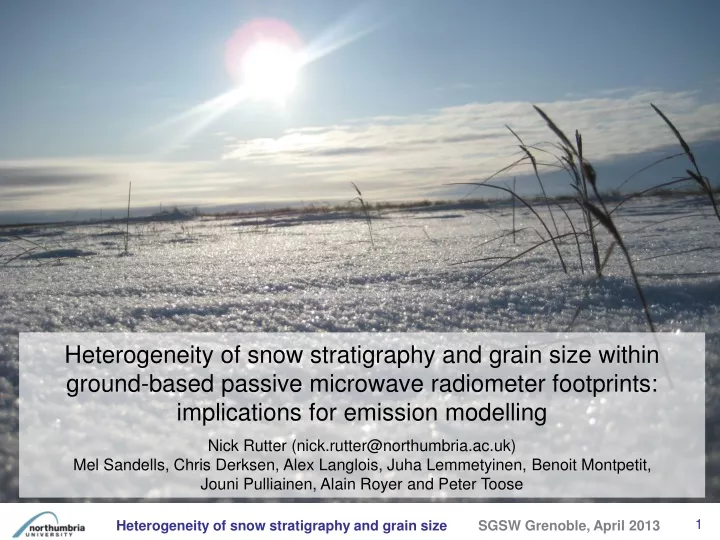
1. Heterogeneity of snow stratigraphy and grain size within ground-based passive microwave radiometer footprints: implications for emission modelling Nick Rutter (nick.rutter@northumbria.ac.uk) Mel Sandells, Chris Derksen, Alex Langlois, Juha Lemmetyinen, Benoit Montpetit, Jouni Pulliainen, Alain Royer and Peter Toose

2. Mel Sandells, ESSC, University of Reading, Reading, U.K. • Chris Derksen and Peter Toose, Environment Canada, Toronto, Canada. • Alain Royer, Benoit Montpetit, Alex Langlois, Université de Sherbrooke, Sherbrooke, Québec, Canada. • Juha Lemmetyinen and Jouni Pulliainen, Finnish Meteorological Institute, Helsinki, Finland. Funding acknowledgements: Many thanks to Environment Canada, University of Waterloo, Canadian Space Agency, European Space Agency and National Centre for Earth Observation.

3. Questions: • What is the spatial variability of snow properties within a footprint? • How does that impact on microwave modelling? • Overview: • Field measurements • Methodological framework: translating 1-D to 2-D • Impact of uncertainty on emission modelling from: • Measurement • Translation • Layering • Grain scaling

4. Location and field site

5. 19 and 37 GHz (dual polarized), uncertainty < 2 K • 1.55 m above snow surface, incidence angle of 53° • Elliptical footprints (13° beam width) far width of 0.29 m and a depth of 0.45 m • ~50% of the power within footprints, ~50% from side lobes • Measurements at 5 sled positions creating overlapping footprints • Vertical profiles (4 cm increments) of physical snow temperatures

6. Excavate trench along centre line of footprints

7. Clean and smooth vertical trench face, set up NIR camera (850 nm) along a rail

8. Take overlapping NIR photos along the face of the trench

9. Try to make background illumination as diffuse as possible!

10. Stitched and geometrically corrected photos allow stratigraphic layer boundaries (resolution: 1 cm scale horizontal, < 1 cm vertical) to be traced from photos along the face of the trench - Tape et al. 2010 and Watts (in prep) • Derksen et al. (2009) showed: • 41 pits across a ~2000 km traverse through NWT and Nunavut (northern Canada) • Average of 6 layers, maximum of 9 layers

11. Sturm and Benson (2004) • Although challenging, this type of snowpack is highly representative of Arctic / sub-Arctic snowpacks approaching maximum SWE • Models need to be working with this level of layer complexity

12. Maximum of 8 layers in any 1-D profile, 17 discrete layers (5 ice lenses)

13. At three positions (75, 185 and 355 cm) along the trench, in situ vertical profiles were made of: • snowpack stratigraphy • density • specific surface area per mass of ice (SSAm). • Specific surface area (SSAm) using a 1310 nm laser with an integrating sphere • deff = 6 / (ρiSSAm)see Gallet et al. (2009) and Montpetit et al. (2012) • where ρi is the density of ice (916 kg m-3 for SSAm given in m2 kg-1)

14. 17 discrete layers (5 ice lenses) • Translate from 1-D to 2-D • Field and NIR stratigraphy are different • singlemeasurements • Multiple measurements use a mean • ice lenses (0.916 g cm-3) • No measurements: subjectivity

15. Snow emission model: Helsinki University of Technology (HUT) • Semi-empirical, multi-layer radiative transfer model (Lemmetyinen et al., 2010) • Parameters: density, grain size and temperature, SWE • Performance of the HUT model assessed at 1 cm horizontal resolution across the entire extent of the sensor footprints. • Vertical profiles of snow and soil information were extracted from this array at each centimetre along the trench to initialize HUT • Twelve brightness temperatures were simulated at each horizontal position: • 19H, 19V, 37H, 37V • Three extinction coefficient models (Hallikainen et al., 1987; Kontu and Pulliainen, 2010; Roy et al., 2004) • This produced a ‘control’ group of brightness temperatures

16. 5 measured Tb for each pol-freq along the length of the trench • Modelled outputs along the trench • Grey area is range using different scattering coefficients • Big changes the result of ice lenses • Lower brightness temperatures were simulated where ice lenses were present • Big Tb differences model – measured • Median brightness temperature simulated was 61K greater than the median of the observations (19 and 37GHz, both polarizations). Model not working in a challenging snowpack. Why?

17. 8 experiments to understand and eliminate potential causes of the bias • Experiments 1 to 5: • 100 simulations were carried out at each vertical profile • Properties of each layer were randomly varied within experimental error • Median trench Tb derived from 45,000 Tb estimates • Experiment 6: • Density of crusts were varied in increments of 50 kg m-3 • Median trench Tb derived from 18,000 Tb estimates

18. Experiment 8: n-layer to 1-layer = 6 K increase in bias

19. Experiment 7: Grain scaling factor (GSF) was increased in increments of 0.1 between 1.5 to 6.0 determine the optimal grain scale factor Bias for optimised runs within measurement error < 2 K

20. From Table 1 in Mätzler (2002) • Scaling factors becoming more common: • Roy et al. (in press): DMRT-ML, GSF = 3.3 • Brucker et al. (2011): DMRT-ML & MEMLS, GSF = 1.89-2.85 • Monpetit et al. (2013): MEMLS, GSF = 1.3 • Langlois et al. (2012): MEMLS with SNOWPACK grains, GSF = 0.1 • Different measurements & modelled grain sizes • GSF is NOT just a free parameter to tune a model • Use GSF as a investigative tool to quantify: • model representation (extinction coefficients) • impact on scattering and emission of grains as assemblages Densified New snow Hard snow and slab Depth hoar

21. Conclusions • New 2-D methodological framework to evaluate snow microwave models • Link heterogeneity in grain assemblages to emission model physics • In this case, the HUT model overestimated the observed brightness temperature with a median bias of 61K • The cause of this bias was not due to measurement uncertainty • Agreement with observations was only obtained through GSF • Is it just HUT? Unlikely - some sample profiles runs with MEMLS have shown only slightly lower biases (~20 to 40K lower depending on model configuration) • Correlation length (Pc) rather than SSA? • MEMLS as a direct input – may give a better agreement with measurements but not the complete answer • SMP or tomography – exciting method but not routinely collected • Methods equally of use for 1) distributed physical snow models (initialisation), 2) data assimilation schemes (variability),and 3) active microwave models

23. Extra Slides

24. Extinction of microwave radiation in snow

26. Translating in-situ measurements from manual to NIR stratigraphies: example using densities • Layers 1 to 9 & 12: direct measurements • Multiple measurements per layer: a mean was used • Layers 13 – 17: ice lenses (0.916 g cm-3) • No layer 10 or 11: subjectivity!

27. Layer 10 assumed a continuation (the mean) of layers 5,8,9

28. Layer 11 assumed same as layer 7 as similar appearance in NIR

29. Same criteria used to translate SSAm profiles to 2-D • Temperature profiles to 2-D: • 5 vertical profiles measured • Create one mean profile • Histogram of layer heights for each layer (from NIR stratigraphy) used to derive a mean height occupied by each layer • Mean layer height attributed to temp at same height on the mean profile • Soil frozen: mean of -2.9 °C