Download
1 / 37
370 likes | 500 Views
Bayesian models for fMRI data. Klaas Enno Stephan Translational Neuromodeling Unit (TNU) Institute for Biomedical Engineering, University of Zurich & ETH Zurich Laboratory for Social & Neural Systems Research (SNS), University of Zurich

E N D
Bayesian models for fMRI data Klaas Enno Stephan Translational Neuromodeling Unit (TNU)Institute for Biomedical Engineering, University of Zurich & ETH Zurich Laboratory for Social & Neural Systems Research (SNS), University of Zurich WellcomeTrust Centre for Neuroimaging, University College London With many thanks for slides & images to: FIL Methods group, particularly Guillaume Flandin and Jean Daunizeau The Reverend Thomas Bayes (1702-1761) SPM Course Zurich 13-15 February 2013
Bayes‘ Theorem Posterior Likelihood Prior Evidence Reverend Thomas Bayes 1702 - 1761 “Bayes‘ Theorem describes, how an ideally rational person processes information." Wikipedia
Bayes’ Theorem Given data y and parameters , the joint probability is: Eliminating p(y,) gives Bayes’ rule: Likelihood Prior Posterior Evidence
Principles of Bayesian inference • Formulation of a generative model likelihoodp(y|) prior distribution p() • Observation of data y • Update of beliefs based upon observations, given a prior state of knowledge
Posterior mean & variance of univariate Gaussians Likelihood & Prior Posterior Posterior: Likelihood Prior Posterior mean = variance-weighted combination of prior mean and data mean
Same thing – but expressed as precision weighting Likelihood & prior Posterior Posterior: Likelihood Prior Relative precision weighting
Same thing – but explicit hierarchical perspective Likelihood & Prior Posterior Posterior Likelihood Prior Relative precision weighting
Why should I know about Bayesian stats? Because Bayesian principles are fundamental for • statistical inference in general • sophisticated analyses of (neuronal) systems • contemporary theories of brain function
Problems of classical (frequentist) statistics p-value: probability of observing data in the effect’s absence • Limitations: • One can never accept the null hypothesis • Given enough data, one can always demonstrate a significant effect • Correction for multiple comparisons necessary Solution: infer posterior probability of the effect
posterior distribution inverse problem Generative models: Forward and inverse problems forward problem likelihood prior
Dynamic causal modeling (DCM) fMRI EEG, MEG Model inversion: Estimating neuronal mechanisms from brain activity measures Forward model: Predicting measured activity given a putative neuronal state Friston et al. (2003) NeuroImage
The Bayesian brain hypothesis & free-energy principle sensations – predictions Prediction error Change predictions Change sensory input Action Perception Maximizing the evidence (of the brain's generative model) = minimizing the surprise about the data (sensory inputs). Friston et al. 2006, J Physiol Paris
IndividualhierarchicalBayesianlearning volatility associations events in the world sensory stimuli Mathys et al. 2011, Front. Hum. Neurosci.
Aberrant Bayesian message passing in schizophrenia: abnormal (precision-weighted) prediction errors abnormal modulation of NMDAR-dependent synaptic plasticity at forward connections of cortical hierarchies Backward & lateral input Forward & lateral Forward recognition effects De-correlating lateral interactions Backward generation effects Lateral interactions mediating priors Stephan et al. 2006, Biol. Psychiatry
Why should I know about Bayesian stats? Because SPM is getting more and more Bayesian: • Segmentation & spatial normalisation • Posterior probability maps (PPMs) • 1st level: specific spatial priors • 2nd level: global spatial priors • Dynamic Causal Modelling (DCM) • Bayesian Model Selection (BMS) • EEG: source reconstruction
Posterior probability maps (PPMs) Spatial priors on activation extent Bayesian segmentation and normalisation Dynamic Causal Modelling Image time-series Statistical parametric map (SPM) Design matrix Kernel Realignment Smoothing General linear model Gaussian field theory Statistical inference Normalisation p <0.05 Template Parameter estimates
Squared distance between parameters and their expected values (regularisation) “Difference” between template and source image Spatial normalisation: Bayesian regularisation Deformations consist of a linear combination of smooth basis functions (3D DCT). Find maximum a posteriori (MAP) estimates: Deformation parameters MAP:
Spatial normalisation: overfitting Affine registration. (2 = 472.1) Template image Non-linear registration without regularisation. (2 = 287.3) Non-linear registration using regularisation. (2 = 302.7)
Bayesian segmentation with empirical priors • Goal: for each voxel, compute probability that it belongs to a particular tissue type, given its intensity • Likelihood: Intensities are modelled by a mixture of Gaussian distributions representing different tissue classes (e.g. GM, WM, CSF). • Priors:obtained from tissue probability maps (segmented images of 151 subjects). p (tissue|intensity) p (intensity|tissue) ∙ p (tissue) Ashburner & Friston 2005, NeuroImage
Bayesian fMRI analyses General Linear Model: with What are the priors? • In “classical” SPM, no priors (= “flat” priors) • Full Bayes: priors are predefined • Empirical Bayes: priors are estimated from the data, assuming a hierarchical generative model Parameters of one level = priors for distribution of parameters at lower level Parameters and hyperparameters at each level can be estimated using EM
Posterior Probability Maps (PPMs) Posterior distribution:probability of the effect given the data mean: size of effectprecision: variability Posterior probability map: images of the probability that an activation exceeds some specified threshold, given the data y • Two thresholds: • activation threshold : percentage of whole brain mean signal • probability that voxels must exceed to be displayed (e.g. 95%)
2nd level PPMs with global priors 1st level (GLM): 2nd level (shrinkage prior): Heuristically:use the variance of mean-corrected activity over voxels as prior variance of at any particular voxel. (1) reflects regionally specific effects assume that it is zero on average over voxels variance of this prior is implicitly estimated by estimating (2) 0 In the absence of evidence to the contrary, parameters will shrink to zero.
2nd level PPMs with global priors 1st level (GLM): voxel-specific 2nd level (shrinkage prior): global pooled estimate over voxels Compute Cε and Cvia ReML/EM, and apply the usual rule for computing posterior mean & covariance for Gaussians: Friston & Penny 2003, NeuroImage
PPMs vs. SPMs PPMs Posterior Likelihood Prior SPMs Bayesian test: Classical t-test:
PPMs and multiple comparisons Friston & Penny (2003): No need to correct for multiple comparisons: Thresholding a PPM at 95% confidence: in every voxel, the posterior probability of an activation is 95%. At most, 5% of the voxels identified could have activations less than . Independent of the search volume, thresholding a PPM thus puts an upper bound on the false discovery rate. NB: being debated
PPMs vs.SPMs PPMs: Show activations greater than a given size SPMs: Show voxels with non-zero activations
PPMs: pros and cons Disadvantages Advantages • One can infer that a cause did not elicit a response • Inference is independent of search volume • do not conflate effect-size and effect-variability • Estimating priors over voxels is computationally demanding • Practical benefits are yet to be established • Thresholds other than zero require justification
Pitt & Miyung (2002) TICS Model comparison and selection Given competing hypotheses on structure & functional mechanisms of a system, which model is the best? Which model represents thebest balance between model fit and model complexity? For which model m does p(y|m) become maximal?
Bayesian model selection (BMS) Model evidence: Gharamani, 2004 p(y|m) y all possible datasets accounts for both accuracy and complexity of the model • Various approximations, e.g.: • negative free energy, AIC, BIC a measure of generalizability McKay 1992, Neural Comput. Penny et al. 2004a, NeuroImage
Approximations to the model evidence Maximizing log model evidence = Maximizing model evidence Logarithm is a monotonic function Log model evidence = balance between fit and complexity No. of parameters In SPM2 & SPM5, interface offers 2 approximations: No. of data points Akaike Information Criterion: Bayesian Information Criterion: Penny et al. 2004a, NeuroImage
The (negative) free energy approximation • UnderGaussianassumptionsabouttheposterior (Laplace approximation):
The complexity term in F • In contrastto AIC & BIC, thecomplexitytermofthe negative freeenergyFaccountsforparameterinterdependencies. • The complexitytermofFishigher • themoreindependentthepriorparameters ( effective DFs) • themoredependenttheposteriorparameters • themoretheposteriormeandeviatesfromthepriormean • NB: Since SPM8, onlyFisusedformodelselection !
Bayes factors To compare two models, we could just compare their log evidences. But: the log evidence is just some number – not very intuitive! A more intuitive interpretation of model comparisons is made possible by Bayes factors: positive value, [0;[ Kass & Raftery classification: Kass & Raftery 1995, J. Am. Stat. Assoc.
M3 attention M2 better than M1 PPC BF 2966 F = 7.995 stim V1 V5 M4 attention PPC stim V1 V5 BMS in SPM8: an example attention M1 M2 PPC PPC attention stim V1 V5 stim V1 V5 M3 M1 M4 M2 M3 better than M2 BF 12 F = 2.450 M4 better than M3 BF 23 F = 3.144