Download
1 / 10
100 likes | 124 Views
Variational Bayesian Inference for fMRI time series. Will Penny, Stefan Kiebel and Karl Friston Wellcome Department of Imaging Neuroscience, University College, London, UK. Generalised Linear Model. A central concern in fMRI is that the errors from scan n-1 to scan n are serially correlated

E N D
Variational Bayesian Inferencefor fMRI time series Will Penny, Stefan Kiebel and Karl Friston Wellcome Department of Imaging Neuroscience, University College, London, UK.
Generalised Linear Model • A central concern in fMRI is that the errors from scan n-1 to scan n are serially correlated • We use Generalised Linear Models (GLMs) with autoregressive error processes of order p yn = xn w + en en= ∑ ak en-k + zn where k=1..p. The errors zn are zero mean Gaussian with variance σ2.
Variational Bayes • We use Bayesian estimation and inference • The true posterior p(w,a,σ2|Y) can be approximated using sampling methods. But these are computationally demanding. • We use Variational Bayes (VB) which uses an approximate posterior that factorises over parameters q(w,a,σ2|Y) = q(w|Y) q(a|Y) q(σ2|Y)
Variational Bayes • Estimation takes place by minimizing the Kullback-Liebler divergence between the true and approximate posteriors. • The optimal form for the approximate posteriors is then seen to be q(w|Y)=N(m,S), q(a|Y)=N(v,R) and q(1/σ2|Y)=Ga(b,c) • The parameters m,S,v,R,b and c are then updated in an iterative optimisation scheme
Synthetic Data • Generate data from yn = x w + en en= a en-1 + zn where x=1, w=2.7, a=0.3, σ2=4 Compare VB results with exact posterior (which is expensive to compute).
Synthetic data True posterior, p(a,w|Y) VB’s approximate posterior, q(a,w|Y) VB assumes a factorized form for the posterior. For small ‘a’ the width of p(w|Y) will be overestimated, for large ‘a’ it will be underestimated. But on average, VB gets it right !
Synthetic Data Autoregressive coefficient posteriors: Exact p(a|Y), VB q(a|Y) Regression coefficient posteriors: Exact p(w|Y), VB q(w|Y) Noise variance posteriors: Exact p(σ2|Y), VB q(σ2|Y )
fMRI Data Event-related data from a visual-gustatory conditioning experiment. 680 volumes acquired at 2Tesla every 2.5 seconds. We analyse just a single voxel from x = 66 mm, y = -39 mm, z = 6 mm (Talairach). We compare the VB results with a Bayesian analysis using Gibbs sampling. Modelling Parameters Y=Xw+e 9 regressors AR(6) model for the errors VB model fitting: 4 seconds Gibbs sampling: much longer ! Design Matrix, X
fMRI Data Posterior distributions of two of the regression coefficients
Summary • Exact Bayesian inference in GLMs with AR error processes is intractable • VB approximates the true posterior with a factorised density • VB takes into account the uncertainty of the hyperparameters • Its much less computationally demanding than sampling methods • It allows for model order selection (not shown)