Download
1 / 59
590 likes | 593 Views
Sinéad M. Farrington University of Liverpool University of Edinburgh Seminar October 2006. B s Mixing at CDF. 0. Lord Kelvin. -. "Science is bound, by the everlasting vow of honour, to face fearlessly every problem which can be fairly presented to it.".

E N D
Sinéad M. Farrington University of Liverpool University of Edinburgh Seminar October 2006 Bs Mixing at CDF 0
Lord Kelvin - "Science is bound, by the everlasting vow of honour, to face fearlessly every problem which can be fairly presented to it." “There is nothing new to be discovered in physics now. All that remains is more and more precise measurement.” (1900) 2
James Clerk Maxwell - “Aye, I suppose I could stay up that late.” 3
Observation of Bs Mixing - • This year the phenomenon of mixing was observed for the first time • in the Bs meson system • I shall: • Describe, in brief, the CDF experiment • Explain why Bs mixing is interesting • Explain the experimental method to measure it • Present the experimental results • Show how these are interpreted within the Standard Model 4
Ecom=2TeV - p CDF p Ep=0.96TeV Ep=0.96TeV 1km D0 ECoM=2TeV The Tevatron - Fermilab, Chicago Currently the world’s highest energy collider Hadron collisions can produce a wide spectrum of b hadrons (in a challenging environment) Bs cannot be produced at the B factories since their Centre of Mass energy is below threshold (except for a special run by Belle) 5
This analysis: Feb 2002 – Jan 2006: 1 fb-1 Recorded Luminosity 1.6 fb-1 Run I: 1992-1996 L= 0.1fb-1 Major Upgrades1996-2001 Run II: 2001-2006 L= 1.6 fb-1 Tevatron Integrated Luminosity
p p The CDF Detector and Triggers • (bb) << (pp) B events are selected with specialised triggers • Displaced vertex trigger exploits long lifetime of B’s • Yields per pb-1 are ~3x those of Run I 7
MATTER ANTIMATTER b b u, c, t, ? s b s s s b Bs Bs Bs 0 0 0 Bs 0 u,c,t,? 0 Bs Physics Bound states: Matterantimatter: NEW PHYSICS? Vts* occurs via W+ W- Vts 0 0 • Physical states, H and L, evolve as superpositions of Bs and Bs • System characterised by 4 parameters: • masses: mH, mL lifetimes: GH, GL(G=1/t) • Predicted Dms around 20ps-1 • No measurements of Dms have been made until now: • B factories do not produce Bs Mesons • Limits set by LEP, SLD, Tevatron "I have no satisfaction in formulas unless I feel their numerical magnitude." (Kelvin)
from Dmd Lower limit on Dms from Dmd/Dms Why ismsinteresting? • Probe of New Physics - may enter in box diagrams 2) Measure CKM matrix element: Dmdknown accurately from B factories • Vtd known to 15% • Ratio Vtd/VtsDmd/Dms related by constants: • (from lattice QCD) known to ~4% • So: measure Dms gives Vts • CKM Fit result: Dms: 18.3+6.5 (1s) : +11.4 (2) ps-1 Standard Model Predicts rate of mixing, Dm=mH-mL, so Measure rate of mixing Vts (or hints of NEW physics) 9
Measuring ms In principle: Measure asymmetry of number of matter and antimatter decays: In practice: asymmetry is barely discernible after experimental realities: After momentum, time resolution, flavour tag power Perfect resolutions 10
Measuring ms So instead we employ two methods: 1:amplitude scan method • Introduce Amplitude, A, to mixing probability formula • Evaluate A at each Dm point • A=1 if evaluated at correct Dm • This method facilitates limit setting before mixing signal observed Mixing signal manifests itself as points in the plot which are most compatible with A=1 H. G. Moser, A. Roussarie, NIM A384 (1997) Test Case: B0d mixing world average 11
Measuring ms 2: To establish the value of Dms, we evaluate the likelihood profile: Log L(A=0)-Log L(A=1) 12
Mixing Ingredients 1) Signal samples - semileptonic and hadronic modes Time of Decay - and knowledge of Proper decay time resolution 3) Flavour tagging - opposite side (can be calibrated on B0 and B+) - same side (cannot be calibrated on B0 and B+, used for the first time at CDF) 14
L Hadronic: fully reconstructed 1) Signal Samples for BsMixing Semileptonic: partially reconstructed These modes are flavour specific: the charges tag the B at decay Crucial: Triggering using displaced track trigger (Silicon Vertex Trigger) 15
Triggering On Displaced Tracks • trigger Bs→ Ds-, Bs→ Ds- l+ Secondary Vertex Primary Vertex d0 Online accuracy • trigger processes 20 TB /sec • trigger requirement: • two displaced tracks: • (pT > 2 GeV/c, 120 m<|d0|<1mm) • requires precision tracking in silicon • vertex detector
Now we use the entire range, capitalising on satellites also Previous mixing fit range Example Hadronic Mass Spectrum signal Bs→ Ds, Ds→ → K+K- partially reconstructed B mesons (satellites) combinatorial background B0→ D- decays
Hadronic Signal Yields • Neural Network selection used in these modes • Particle ID (dE/dx, Time of Flight) used to suppress backgrounds
Semileptonic Samples: Ds- l+ x Bs mesons not fully reconstructed: Fully reconstructed Ds mesons: Mixing fit range Particle ID used; new trigger paths added The candidate’s m(lDs-) is included in the fit: discriminates against “physics backgrounds” of the type B0/+→ D+Ds 61500 semileptonic candidates
Summary of Yield changes since April 2006 • 1fb-1 of data used in both analyses • What changed? • Hadronic modes: • Added partially reconstructed “satellite” Bs decays • Add Neural Net for candidate selection • Used particle identification to eliminate background • Semileptonic Modes: • Used particle identification to eliminate background • Added new trigger path Effective increase in statistics x2.5 from these changes
850 Per Bs meson What do the candidates cost?: FECb Tevatron Accelerator Value: $7M/year ($741M RPV at 70% spread over 25 years and 3 experiments) CDF Detector Value: $0.8M/year ($95M total facilities RPV at 70% value) Tevatron Operation to CDF: $48M/year ($120M/year at 40% of overall facilities) CDF Operation: $5M/year Total CDF data $61M/year B Physics Program: $12M/year (1/5 per physics group) 0 The Bsottom Line: $ 21
osc. period at ms = 18 ps-1 2) Time of Decay • Reconstruct decay length by vertexing • Measure pT of decay products Proper time resolution: Semileptonic: Hadronic: Crucial: Vertex resolution (Silicon Vertex Detector, in particular Layer00 very close to beampipe) 22
Layer 00 • So-called because we already had layer 0 when this device was designed! • UK designed, built and (mostly) paid for this detector! • layer of silicon placed directly on beryllium beam pipe • Radius of 1.5 cm • additional impact parameter resolution I.P resolution without L00
B decays pp collision Classic B Lifetime Measurement • reconstruct B meson mass, pT, Lxy • calculate proper decay time (ct) • extract c from combined mass+lifetime fit • signal probability: psignal(t) = e-t’/ R(t’,t) • background pbkg(t) modeled from sidebands
Hadronic Lifetime Measurement • Displaced track trigger biases the lifetime distribution • Correct with an efficiency function derived from MC: p = e-t’/ R(t’,t) (t) 0.2 0.4 0.0 proper time (cm)
Hadronic Lifetime Measurements Errors are statistical only World Averages: B0: 1.534 ± 0.013 ps B-: 1.653 ± 0.014 ps Bs: 1.469 ± 0.059 ps Good agreement in all modes
Semileptonic Lifetime Measurement • neutrino momentum missing • Correct with “K factor” from MC: • Also correct for displaced track trigger bias as in hadronic case High m(lD) candidates have narrow K factor distribution: almost fully reconstructed events! Capitalise on this by binning K factor in m(lD)
Lepton+Ds Lifetime Fits Two cases treated separately: Lepton is a displaced track: Lepton is not a displaced track:
Errors are statistical only Lifetimes measured on first 355 pb-1 Compare to World Average: Bs: (1.469±0.059) ps All Lifetime results are consistent with world average Gives confidence in fitters, backgrounds, ct resolution Semileptonic Lifetime Results
jet charge p soft lepton fragmentation K b hadron f Bs Ds Opposite side Same Side p- To determine B flavour at production, use tagging techniques: 3) Flavour Tagging b quarks produced in pairs only need to determine flavour of one of them OPPOSITE SIDE Soft Muon Tag semileptonic BR ~10% Soft Electron Tag Jet charge tagsum of charges in jet eD2 =1.82±0.04 % (semileptonic) 1.81±0.10 % (hadronic) SAME SIDE Same Side K Tag eD2 = 4.8±0.04 %(semileptonic) 3.5±0.06 % (hadronic) Figure of merit is eD2e = efficiency (% events tagger can be applied) D = dilution (% events tagger is correct) 30 Crucial: Particle Identification (Time of Flight Detector)
Opposite Side Taggers • Performance studied in high statistics inclusive lepton+SVT trigger • Enables calibration of taggers • Can also parameterise tagging dilution as function of variables: • Soft Lepton Tag: dilution parameterised as function of • likelihood and ptrel • Jet Charge Tag: dilution parameterised as function of jet charge • for a given jet Soft Electron Tag Soft Electron Tag Jet Charge Tag 31
b b s } s u u K+ Bs 0 • This is the first time this type of tagger has been implemented • Principle: charge of B and K correlated • Use TOF, dE/dx to select track • Tagger eD2 not measurable in data until Bs mixing frequency known Same Side (Kaon) Tagger b hadron 32
CDF Public Note 8206 • If MC reproduces distributions well for B0,B+, then rely on it to extract tagger power in Bs (with appropriate systematic errors) • High statistics B0 and B+ samples in which to make data/MC comparisons: • Systematics: production mechanism, fragmentation model, particle fraction around B, PID simulation, pile-up, MC/data agreement Same Side (Kaon) Tagger B0d Kaon enhanced B0s 33
Summary of Tagging changes since April 2006 • What changed? • Opposite Side Taggers: • Added new tagger: Opposite Side Kaon Tagger • New method to combine opposite side tags • Before, it was hierarchical • Now combination is performed by neural net • Every tagger can contribute some power • Same Side Kaon Tagger: • Neural Net used to incorporate kinematic information as well • as particle identification
The Results 35
Amplitude scan performed on Bs candidates • Inputs for each candidate: • Mass • Decay time • Decay time resolution • Tag decisions • Predicted dilution • Mass(lepton+D) if semileptonic Put the 3 Ingredients Together • All elements are then folded into the amplitude scan “With three parameters, I can fit an elephant.” (Kelvin) 36
A Priori Procedure Decided upon before un-blinding the data: (everything blinded so far by scrambling tagger decision) • Find highest significant point on amplitude scan consistent with an amplitude of 1 • significance to be estimated using (log Likelihood) method • effectively infinite Dms search window to be used Is probability for “signal” to be a fluctuation < 1%? NO YES make double-sided confidence interval from Dlog(Likelihood) Measure ms (Since we already had <1% probability in April we weren’t expecting to follow this route in September with the improved analysis) set 95% CL limit based on Amplitude Scan
Systematic Uncertainties Semileptonic Decays • related to absolute value of amplitude, relevant only when setting limits • cancel in A/A, folded in to confidence calculation for observation • systematic uncertainties are very small compared to statistical
Combined Amplitude Scan Amplitude consistent with 1 at Dms ~17.75ps-1: 1.21±0.20(stat) (and inconsistent with 0) How significant is this result?
Separate Samples …but the hadronic analysis gives a clear signature of mixing even on its own! World best semileptonic analysis with sensitivity of 19.3ps-1 40
Likelihood Ratio Profile How often can random tags produce a likelihood dip this deep?
Likelihood Significance • probability of fake from random tags = 8x10⁻⁸measure ms • Equivalent to 5.4s significance ms = 17.77±0.10(stat)±0.07(syst) ps-1
Systematic Uncertainties on ms • Systematic uncertainties from fit model evaluated on toy Monte Carlo • Have negligible impact • Relevant systematic uncertainties are from lifetime scale All systematic uncertainties are common between hadronic and semileptonic samples
Asymmetry Oscillations folded modulo 2p/Dms
|Vts| / |Vtd| • Can extract Vts value • compare to Belle bs(hep-ex/050679): |Vtd| / |Vts| = 0.199 +0.026 (exp) +0.018 (theo) • our result: |Vtd| / |Vts| = 0.2060 ± 0.0007(exp) +0.0081 (theo) -0.025 -0.016 -0.0060 • inputs: • m(B0)/m(Bs) = 0.9832 (PDG 2006) • = 1.21 +0.05 (Lattice 2005) • md = 0.507±0.005 (PDG 2006) -0.04
Interpretation of Results Measurements compared with global fit (CKM fitter group) updated this month In excellent agreement with expectations
Interpretation of Results This measurement decreases uncertainty on CKM triangle apex: October 2006 Easter 2006
"There is nothing more practical than a good theory." Vts / Vtd= 0.2060 ± 0.0007 (exp) +0.0081 (theo) -0.0060 Conclusions • CDF has found a signature consistent with Bs - Bs oscillations • Probability of this being a fluctuation is 8x10⁻⁸ • Presented direct measurement of the Bs - Bs oscillation frequency: ms = 17.77±0.10(stat)±0.07(syst) ps-1
prompt track Ds- vertex “Bs” vertex P.V. Proper Time Resolution • Displaced track triggers also gather large prompt charm samples • construct “Bs-like” topologies of prompt Ds- + prompt track • calibrate ct resolution by fitting for “lifetime” of “Bs-like” objects • expect zero lifetime by construction trigger tracks
osc. period at ms = 18 ps-1 • utilize large prompt charm cross section • construct “Bs-like” topologies of prompt Ds- + prompt track • calibrate ct resolution by fitting for “lifetime” of “Bs-like” objects Proper Time Resolution • event by event determination of primary vertex position used • average uncertainty ~ 26 m • this information is used per candidate in the likelihood fit semileptonic: hadronic: 50