Download
1 / 23
230 likes | 312 Views
Meas urement of B s oscillations at CDF. Giuseppe Salamanna Univ. di Roma “La Sapienza” & INFN Roma for the CDF Collaboration. BEACH 2006 July 2006 Lancaster (UK). Outline.

E N D
Measurement of Bs oscillations at CDF Giuseppe Salamanna Univ. di Roma “La Sapienza” & INFN Roma for the CDF Collaboration BEACH 2006 July 2006 Lancaster (UK)
Outline • Motivations: ΔMs and the Unitarity Triangle • Analysis details: • Trigger and reconstruction • Lifetime measurements and biases • Flavour tagging • (Some) Statistical details and expected significance • Results for ΔMs • Interpretation and derived constraints • Paper submitted to PRL: hep-ex/0606027
Why ΔMs Observation of a quantum phenomenon: flavour oscillations via a ΔF = 2 Box diagram • The only relevant diagram has b coupling with top • New (s)particles in the loop..? Form factors and B-parameters from Lattice calculations have high uncertainty → Vtd known only at ~15% level Mixing involves CKM elements → measuring ΔMq constraints the unitarity triangle
UT and constraint from mixing • From lattice: • Ratio ≡ ξ2 is better • calculated than single factors • ξ = 1.210 + 0.047-0.035(M.Okamoto, hep-lat/0510113) • ♣ Measuring ΔMs /ΔMd returns Vts / Vtd with ~4% error from theory ΔMd only Limit on ΔMs ΔMs /ΔMd • UP TO WINTER ‘06: • ΔMs ≥ 16.6 ps-1(LEP+SLD+Tevatron I and II) • Expected value (UT fit, utfit.roma1.infn.it): • ΔMs (SM) = 21.5 ± 2.6 ps -1 • ΔMs in [16.7, 26.9] @ 95% CL • ♣LARGER ΔMs could indicate NP contrib’s
Want to measure…so, how? • Final state: • Reconstruct final states from both Semileptonic (high statistics, but missing kinematics) and Hadronic (fully reconstructed, best ct resolution) • Lifetime measurement • Hadronic decay length measured with better resolution than Semileptonic • Flavour tagging • Tag the flavour of the mixing B candidate using both: • correlation with fragmentation tracks AND • flavour of other b (incoherentb-b production)
Introduce “Amplitude” in Likelihood Amplitude Scan • Fit A for fixed ΔM • A consistent with: • 1 if mixing detected at a given ΔM • 0 if no mixing at a given ΔM • Limit where A+1.645σA = 1 • Sensitivity: 1.645σA = 1 Example of amplitude scan World Average, Fall ‘05
Measurement significance Trigger-challenge to collect S suppressing B • The expression of the statistical Significance of a mixing measurement is given by: Signal (b-flavour at decay tagged) Experimental time resolution exponentially dilutes a measurement Fraction of S with info also on flavour at creation • Significance exponentially reduced at higher ΔMs … • …|Vts| >> |Vtd| Ms ~40·Md
“Satellites”: (Not used in this analysis) Hadronic signals • Fully reconstructed decays triggered on • at CDF only; requiring 2 tracks with • d0 > 120 μm(τ(B)≈1.5ps) • Pt > 5.5 GeV/c L = 1 fb-1 N(Bs) ≈ 3600 Bs0→ Ds-(3)π+ (Ds- → φπ-, φ→ K+ K-)
Semileptonic signals Bs0→ Ds-(*)ℓ+νX (Ds- → φπ-) • Missing Pt→ No Bs mass peak • Use Ds mass signals • Using M(lDs) helps bkg rejection • Charge correlation between ℓ and Ds: • Bkg also from Right Sign (~15%): • Ds + fake lepton from PV • Bs,d to DsDX, D to ℓ νX • cc background ~37000 semileptonic Bs candidates
Hadronic Lifetime Results • World Average (HFAG06) • cτ(B+) = 491.1 ± 3.3(stat) μm • cτ(Bd) = 458.7 ± 2.7 μm • Bs→Flavour specific: • cτ(Bs) = 432 ± 20 ps • Detailed simulation to correct for • trigger bias • on the selection of the B decay length • Syst. on trigger efficiency negligible • for mixing measurements Excellent agreement !
Amplitude of mixing asymmetry diluted by a factor Effect of proper time resolution Vertex resolution (constant) Momentum resolution (~ct) Semileptonic-like <σp/p> ≈15% CDF II osc. period at Ms = 18 ps-1 Hadronic-like • Calibrated on large D+ data samples combined with • prompt tracks to mimic B0-like topologies • Calibrate by fitting for lifetime of B0-like decays
Combined tagging power • Opposite Side Taggers (OST) tag the other b-hadron in the event using e and μ from decay and jet charge • Combine OST exclusively • Calibrate Combined OST on samples of B+ and Bd (by measuring ΔMd) • Add Same Side Kaon Tagger independently Dilution = 1-2•mistag rate Efficiency
Bs K- K*0 Main “boost” is from SSKT • Exploits the charge correlation between the b flavour and the leading product of b hadronization • Close to trigger B: large acceptance! • SSKaon Tagging exploits PID over wide momentum range → use a combined TOF+dE/dxlikelihood ratio • Dilution depends on the fragmentation process → cannot calibrate using Bd and B+ → Need to estimate D from MC • Extended MC-data comparison on quantities related to fragmentation • Then test predictions on data for other species (B+ and Bd) and add systematics on agreement accordingly for usage with Bs
Amplitude Scan (hadronic+semileptonic) A/A (17.3 ps-1) = 3.7
CDF II 1 fb-1 -0.45 ± 0.23 (25.8 ps-1) Sensitivity • CDF sensitivity compared to WA • Use the Likelihood Ratio: • -Δlog(L) = -log[ L(A=1) / L(A=0) ] • to evaluate the probability p of null experiment (bkg fluctuations) • This sensitivity reached with: • 1 fb-1 • Addition of SSKT • Improved σct fitting model
Significance of the peak • From data • –Δlog(L)MIN = -6.75 • Randomize tags ~50k • times on data and • calculate…. • P-value = 0.2% • Significance > 3σ • → assume that peak • IS real mixing signal
Finally….ΔMs • Contribution of hadronic modes • essential due to better • ct resolution at high ΔMs • σ(ΔMs)/ ΔMs~ 0.02 • ms in [17.01, 17.84] ps-1 at 90% CL • ms in [16.96, 17.91] ps-1 at 95% CL • Systematics low and under control: • dominated by uncertainty on the • absolute scale of the decay-time • measurement
From ΔMs :information on UT • Compatible with SM • within 1σ • From measurement and chosen inputs • (m(B0)/m(Bs) = 0.9830, ΔMd = 0.505 ± 0.005 ps-1 • from PDG06 and • ξ = 1.210+ 0.047 -0.035, hep-lat 0510113) • we infer the value: • |Vtd|/|Vts| = 0.208 +0.001 -0.002 (exp) +0.008-0.006(th) • Constraint on CBs: • CBs = MsSM+NP/MsSM = 1.01 0.33 • [0.33,2.04] @ 95% CL (UTFit, utfit.roma1.infn.it)
Conclusions… • CDF finds signature consistent with Bs oscillations • Probability of fluctuation from random tags is 0.2% • Constraints to UT: • ρ = 0.193 ± 0.029 (was 0.240 ± 0.037 ) • η = 0.355 ± 0.019 (was 0.333 ± 0.022 ) (UTFit) • …and perspectives • Inclusion of partially reconstructed decays • Refinement of fully reconstructed mode selections to gain events • New OS Kaon Tagger in place: εD2 = 0.23 ± 0.02 %