Download
1 / 62
620 likes | 765 Views
Link Layer: Wireless Mesh Networks Capacity. Y. Richard Yang 11 /13/2012. Outline. Admin. and recap Wireless mesh network capacity Maximize mesh capacity. Admin. Exam Average (mean): 68.6; max = 74 Project check point 1 Sending email to cs434ta@cs.yale.edu Includes contents on

E N D
Link Layer:Wireless Mesh Networks Capacity Y. Richard Yang 11/13/2012
Outline • Admin. and recap • Wireless mesh network capacity • Maximize mesh capacity
Admin. • Exam • Average (mean): 68.6; max = 74 • Project check point 1 • Sending email to cs434ta@cs.yale.edu • Includes contents on • references • setting
Recap: Wireless Link Access Control • Problem: single shared medium, hence if two transmissions overlap on all dimensions [time, space, frequency, and code], then it is a collision Slotted ALOHA Ethernet Hidden-terminalCollision detection/prevention Zigzag decoding
B1 = 25 wait data data wait B2 = 10 B2 = 20 Recap: 802.11 CSMA/CA busy B1 = 5 B2 = 15 busy B1 and B2 are backoff intervals at nodes 1 and 2 cw = 31
∆2 Recap: ZigZag Decoding Exploits 802.11’s behavior • Retransmissions Same packets collide again • Senders use random jitters Collisions start with interference-free bits ∆1 Pa Pa Pb Pb Interference-free Bits
∆2 ZigZag Algorithm 1 1 ∆1 ∆1 ≠∆2 while (exists a chunk that is interference-free in one collision and has interference in the other) { decode and subtract from the other collision }
∆2 How Does ZigZag Work? 1 1 ∆1 2 ∆1 ≠∆2 while (exists a chunk that is interference-free in one collision and has interference in the other) { decode and subtract from the other collision }
∆2 How Does ZigZag Work? 3 1 ∆1 2 2 ∆1 ≠∆2 while (exists a chunk that is interference-free in one collision and has interference in the other) { decode and subtract from the other collision }
∆2 How Does ZigZag Work? 3 3 1 ∆1 2 4 ∆1 ≠∆2 while (exists a chunk that is interference-free in one collision and has interference in the other) { decode and subtract from the other collision }
∆2 How Does ZigZag Work? 5 3 1 ∆1 4 2 4 ∆1 ≠∆2 while (exists a chunk that is interference-free in one collision and has interference in the other) { decode and subtract from the other collision }
∆2 How Does ZigZag Work? 5 3 5 1 ∆1 2 6 4 ∆1 ≠∆2 while (exists a chunk that is interference-free in one collision and has interference in the other) { decode and subtract from the other collision }
∆2 How Does ZigZag Work? 7 5 3 1 ∆1 6 2 6 4 ∆1 ≠∆2 while (exists a chunk that is interference-free in one collision and has interference in the other) { decode and subtract from the other collision }
∆2 How Does ZigZag Work? 7 5 3 7 1 ∆1 2 8 6 4 ∆1 ≠∆2 while (exists a chunk that is interference-free in one collision and has interference in the other) { decode and subtract from the other collision } Delivered 2 packets in 2 timeslots As efficient as if the packets did not collide
Implementation • USRP Hardware • GNURadio software • Carrier Freq: 2.4-2.48GHz • BPSK modulation
Testbed USRPs • 10% HT, • 10% partial HT, • 80% perfectly sense each other 802.11a
Throughput Comparison Perfectly Sense Partial Hidden Terminals Hidden Terminals CDF of concurrent flow pairs 802.11 Throughput
Throughput Comparison ZigZag Exploits Capture Effect Hidden Terminals get high throughput CDF of concurrent flow pairs ZigZag 802.11 Throughput
∆2 ∆1 Capture Effect • Subtract Alice and combine Bob’s packet across collisions to correct errors Pa1 Pa2 Pb Pb 3 packets in 2 time slots better than no collisions
Summary Basic lesson: Traditional thinking was on avoiding collisions Zigzag changed the way of thinking: decoding collisions Many extensions of the Zigzag idea: decoding collisions, instead of avoiding collisions See Remap in Backup Slides 20
Infrastructure Mode Wireless 802.11 by default operates in infrastructure mode. AP wired network AP: Access Point AP AP Problems of infrastructure mode wireless networks?
Mesh Networks AP wired network AP: Access Point AP AP • fast and low-cost deployment • no central point of failure • no APs overhead for users who can reach each other ad-hoc (mesh) mode
Outline • Admin. and recap • Wireless mesh network capacity
Capacity of Mesh Networks • The question we study: how much traffic can a mesh wireless network carry, assuming an oracle to avoid the potential overhead of distributed synchronization (MAC)? • Why study capacity? • learn the fundamental limits of mesh wireless networks • separate the spatial reuse perspective and system design perspective • gain insight for designing effective wireless protocols
receiver r (1+D)r sender Mesh Transmission Constraints Radio interface constraint Interference constraint • a single half-duplex transceiver at each node: • either transmits or receives • transmits to only one receiver • receives from only one sender • transmissionsuccessful if there areno other transmitterswithin a distance (1+D)rof the receiver
Model • Domain is a disk of unit area • There are n nodes in the domain • The transmission rate is W bits/sec
Capacity of Mesh Wireless Network • Consider two types of networks • arbitrary networks: place nodes optimally to derive overall upper bound • random network: nodes are placed randomly
Outline • Admin • Wireless mesh network capacity • setting • arbitrary networks: place nodes optimally to derive overall upper bound
1 1 2 2 3 3 4 4 5 5 bit time 1 bit time WT bit time 2 bit time t Transmission Model: Bit-time Perspective • Chop time into a total of WT bit-times in T seconds • The transmission decision is made for each bit
Transmission Model: End-to-end Perspective • Assume the network sends a total of T end-to-end bits in T seconds • Assume the b-th bit makes a total of h(b) hops from the sender to the receiver • Let rbh denote the hop-length of the h-th hop of the b-th bit 1 2 T 2
2 Hop-Count Constraint Since there are a total of WT bit-times, and during each bit-time there are at most n/2 simultaneous transmissions, we have
(1+)r’ (1+)r m ½ r r’ k j r i Area Constraint • Consider two simultaneoustransmissions at a bit-time ½ r’ Djm + r >= Dim >= (1+)r’ Djm + r’ >= Djk >= (1+)r Djm >= (r+r’) /2
Area Constraint • For each transmissionwith distance r from sender to receiver, we draw a circle with radius ½ r • These circlesdo not overlap
sum over all circles, since each circle has at least ¼ of its area in the unit disk, Area Constraint: Global Picture 2
receiver r (1+D)r sender Summary: Two Constraints Radio interface constraint Interference constraint • a single half-duplex transceiver at each node • transmissionsuccessful if there areno other transmitterswithin a distance (1+D)rof the receiver
Discussion: what does the result mean? Capacity Bound Note: Let L be the average (direct-line) distance for all T end-to-end bits.
Discussion • L depends on • traffic pattern (who needs to talk to whom) and • positions of the end-to-end (application-level) senders and (application-level) receivers • If end-to-end senders and receivers are spread out throughout the network, L is large • per node capacity • Otherwise, L will be small as network becomes denser
Achieving Capacity: Example • n/2 senders and receivers: • L=
Results: Arbitrary Networks Protocol Model
Outline • Admin • Wireless mesh capacity • setting • arbitrary networks: place nodes optimally to derive overall upper bound • random networks: uniform distribution of nodes andsenders/receivers
Uniform Random Networks • Uniform distribution of n nodes • n origin-destination (OD) pairs • Each node chooses same power level P, and thus equal radius r(n) • Equal throughput (n)bits/sec for all ODpairs
Random Networks: Required Bits • Assume: average length of each OD pair is L • Average number of hops: • Total required bit transmissions per second to support l(n):
Random Networks: Offered Bits • Required bit transmissions per second: • What is the maximum number of transmissions (of bits) in one second? • space used per transmission (interference limited): • at least ¼ p [Dr(n)/2]2 = pD2r2(n)/16 • number of simultaneous transmissions at most (interference limited): • total bits per second
Random Networks: Capacity Required ≤ offered
Connectivity Constraint • Need routes between origin-destination pairs - places a lower bound on transmit range r(n) A A D D Connected Not connected To maintain connectivity with a high probability, requires r(n) on the order:
Random Networks: Capacity Required ≤ offered
Measured scaling law: throughput declines worse with n than theoretically predicted: 1/n1.68 Remaining story line wireless mesh networks may have low scalability, and need techniques to increase capacity Measurement
Improving Wireless Mesh Capacity Radio interface constraint Interference constraint • a single half-duplex transceiver at each node • transmissionsuccessful if there areno other transmitterswithin a distance (1+D)rof the receiver Reduce L Increase W Approx.optimal rate*distance capacity: Multipletransceivers Reduceinterf. area
Outline • Admin. and recap • Wireless mesh network capacity • Maximize mesh capacity • Reduce L