Download
1 / 117
1.27k likes | 1.58k Views
Wireless Ad Hoc & Sensor Networks. Nordic Radio Symposium 2004 August 16 – 18, 2004 University of Oulu, Finland Presenter: Carlos Pomalaza-Ráez carlos@ee.oulu.fi http://www.ee.oulu.fi/~carlos/NRS_04_Tutorial.ppt. Outline. Mobile Ad Hoc Networks (MANETs) Main features

E N D
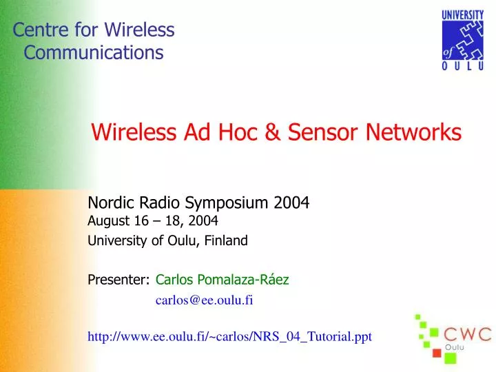
Wireless Ad Hoc & Sensor Networks Nordic Radio Symposium 2004August 16 – 18, 2004 University of Oulu, Finland Presenter:Carlos Pomalaza-Ráez carlos@ee.oulu.fi http://www.ee.oulu.fi/~carlos/NRS_04_Tutorial.ppt
Outline • Mobile Ad Hoc Networks (MANETs) • Main features • Very brief discussion of graph theory, shortest path algorithms, and routing algorithms • Wireless Sensor Networks • Main features • Energy model • WSN protocols • Final Words
Mobile Ad Hoc Networks (MANET) A loose collection of mobile nodes that are capable of communicating with each other without the aid of any established infrastructure or centralized administration • Main Features • Dynamic topology • Each node acts as an independent router • Because of the wireless mode of communication: • Bandwidth-constrained and variable capacity links • Limited transmitter range • Energy-constrained • Limited physical security • MAC and network protocols are of a distributed nature • Complex routing protocols with large transmission overheads and large processing loads on each node
Dynamic Topology Node mobility has a great effect on the designing of routing protocols Node mobility creates a dynamic topology, i.e., changes in the connectivity between the nodes
Graph Theory Application to MANETS • Networks can be represented by weighted graphs • The nodes are the vertices • The communication links are the edges • Edge weights can be used to represent metrics, e.g. cost associated with the communication links Vertices 1 8 5 4 10 2 Edges Weights • Routing protocols often use shortest path algorithms
Shortest Path Algorithms • Assume non-negative edge weights • Given a weighted graph and a nodes, a shortest path tree T rooted at s is a tree such that, for any other node v, the path between s and v in T is a shortest path between the nodes 2 2 2 6 2 6 3 1 3 5 1 2 2 4 4 Shortest Path Spanning Treerooted at vertex 1 Graph • Examples of the algorithms that compute these shortest path trees are Dijkstra and Bellman-Ford algorithms
Distributed Asynchronous Shortest Path Algorithms • Each node computes the path with the shortest weight to every network node • There is no centralized computation • Control messaging is required to distribute the computation • Asynchronous means here that there is no requirement of inter-node synchronization for the computation performed at each node for the exchange of messages between nodes
Routing Protocols • Desired Properties • Distributed • Consider both uni- and bi-directional links • Energy efficient • Secure • Performance Metrics • Data throughput • Delay • Overhead costs • Power consumption
Proactive routing maintains routes to every other node in the network Regular routing updates impose large overheads Suitable for high traffic networks Reactive routing maintains routes to only those nodes which are needed Cost of finding routes is expensive since flooding is involved Good for low/medium traffic networks Proactive vs. Reactive
AODV – Path Finding neighbors re-broadcast the packet until it reaches the intended destination source broadcasts a route request packet S A B RREQ D H reply packet follows the reverse path of the route request packet recorded in broadcast packet RREP C G D node discards packets that have been seen F node discards packets that have been seen E
Traditional Routing Protocols Destination Source Consider several routes Find the best Then use it as much as possible • Problems • Energy depletion in certain nodes • Not suitable for Wireless Sensor Networks
Wireless Sensor Networks What is a sensor? A device that produces a measurable response to a change in a physical or chemical condition, e.g. temperature, ground composition • Sensor Networks • A large grouping of low-cost, low-power, multifunctional, and small-sized sensor nodes • They benefit from advances in 3 technologies: • digital circuitry • wireless communication • silicon micro-machining
Sensing Networking Computation Wireless Sensor Networks (WSNs) New technologies have reduced the cost,size, and power of micro-sensors and wireless interfaces Circulatory Net EnvironmentalMonitoring Structural
Some Applications of WSNs • Battlefield Detection, classification and trackingExamples: AWAIRS (UCLA & Rockwell Science Center) • Habitat Monitoring Micro-climate and wildlife monitoring Examples: • ZebraNet (Princeton) • Seabird monitoring in Maine’s Great Duck Island (Berkeley & Intel)
Some Applications of WSNs • Structural, seismic Bridges, highways, buildings Examples: Coronado Bridge San Diego (UCSD), Factory Building (UCLA) • Smart roads Traffic monitoring, accident detection, recovery assistance Examples: ATON project (UCSD) highway camera microphone • Contaminants detectionExamples: Multipurpose Sensor Program (Boise State University)
WSN Communications Architecture Sensing node Sensor nodes can be data originators and data routers Internet Sink Manager Node Sensor nodes Sensor field
Typical Features of WSNs • A very large number of nodes • Asymmetric flow of information • Communications are triggered by queries or events • At each node there is a limited amount of energy • Almost static topology • Low cost, size, and weight per node • Prone to failures • Broadcast communications instead of point-to-point • Nodes do not have a global ID such as an IP number • Limited security
Design Considerations • Fault tolerance – The failure of nodes should not severely degrade the overall performance of the network • Scalability – The mechanism employed should be able to adapt to a wide range of network sizes (number of nodes) • Cost – The cost of a single node should be kept very low • Power consumption – Should be kept to a minimum to extend the useful life of network • Hardware and software constraints – Sensors, location finding system, antenna, power amplifier, modulation, coding, CPU, RAM, operating system • Topology maintenance – In particular to cope with the expected high rate of node failure • Deployment – Pre-deployment mechanisms and plans for node replacement and/or maintenance • Environment – At home, in space, in the wild, on the roads, etc. • Transmission media – ISM bands, infrared, etc.
Sensor Network Traditional Protocol Stack Power Management – How the sensor uses its power, e.g. turns off its circuitry after receiving a message Topology Management – Detects and registers changes in the positions of the nodes Application Task Management Mobility Management Transport Power Management Network Data Link Task Management – Balances and schedules the sensing tasks given to a specific region Physical
Physical Layer • Frequency selectionISM bands have often been proposed • Carrier frequency generation and signal detectionAim for simplicity, low power consumption, and low cost per unit • ModulationBinary modulation schemes are simpler to implement and thus deemed to be more energy-efficient for WSN applications • Low transmission power and simple transceiver circuitry make Ultra Wideband (UWB) an attractive candidate Application Transport Network Data Link Physical
Physical Layer Energy consumption minimization is of paramount importance when designing the physical layer for WSN in addition to the usual factors such as scattering, shadowing, reflection, diffraction, multipath, and fading
Energy Limitations • Each sensor node has limited energy supply • Nodes may not be rechargeable • Energy consumption in • Sensing • Data processing • Communication (most energy intensive) 20 15 Power (mW) 10 5 0 Sensing CPU TX RX IDLE SLEEP Power consumption of a typical node’s subsystems
Tx Rx Sleep CWC WIRO (WIreless Research Object ) CPU Board 2 Euro coin & RF Board WIRO Box RF Board Total Power Consumption
Node Energy Model A typical node has a sensor system, A/D conversion circuitry, DSP and a radio transceiver. The sensor system is very application dependent. The communication components consume most of the energy.A simple model for a wireless link is:
Energy Model The energy consumed when sending a packet of m bits over a one hop wireless link can be expressed as: Transmitter Receiver where, ET = energy used by the transmitter circuitry and power amplifier ER = energy used by the receiver circuitry PT = power consumption of the transmitter circuitry PR= power consumption of the receiver circuitry Tst = startup time of the transceiver Eencode = energy used to encode Edecode = energy used to decode
Energy Model Assuming a linear relationship for the energy spent per bit at the transmitter and receiver circuitry ET and ER can be written as, where eTC, eTA, and eRC are hardware dependent parameters and αis thepath loss exponent whose value varies from 2 (for free space) to 4 (for multipath channel models). The effect of the transceiver startup time, Tst, will greatly depend on the type of MAC protocol used. To minimize power consumption it is desirable to have the transceiver in a sleep mode as much as possible. However, constantly turning the transceiver on and off to bring it to readiness for transmission or reception also consumes energy.
Energy Model An explicit expression for eTA can be derived as(†), Where, (S/N)r = minimum required signal-to-noise ratio at the receiver’s demodulator for an acceptable Eb/N0 NFRx =receiver noise figure N0 = thermal noise floor in a 1 Hertz bandwidth (Watts/Hz) BW = channel noise bandwidth λ = wavelength in meters α = path loss exponent Gant = antenna gain ηamp = transmitter power efficiency Rbit = raw bit rate in bits per second (†)P. Chen, B. O’Dea, E. Callaway, “Energy Efficient System Design with Optimum Transmission Range for Wireless Ad Hoc Networks,” IEEE International Conference on Comm. (ICC 2002), Vol. 2, pp. 945-952, 28 April -2 May 2002, pp. 945-952.
Energy Model The expression for eTA can be used for those cases where a particular hardware configuration is being considered. The dependence of eTA on (S/N)rcan be made more explicit if the previous equation is written as: This expression shows explicitly the relationship between eTA and (S/N)r. The probability of bit error p depends on Eb/N0 which in turns depends on (S/N)r. Eb/N0is independent of the data rate. In order to relate Eb/N0to (S/N)r, the data rate and the system bandwidth must be taken into account, i.e.,
Energy Model where Eb = energy required per bit of information R = system data rate BT = system bandwidth γb = signal-to-noise ratio per bit, i.e., (Eb/N0) Typical Bandwidths for Various Digital Modulation Methods
Energy Model Power Scenarios Two possible power scenarios are: • Variable transmission power. In this case the radio dynamically adjusts its transmission power so that (S/N)r is fixed to guarantee a certain level of Eb/N0at the receiver. The transmission energy per bit is given by: Since (S/N)r is fixed at the receiver this also means that the probability p of bit error is fixed at the same value for each link.
Fixed transmission power. In this case the radio uses a fixed power for all transmissions. This case is considered because several commercial radio interfaces have a very limited capability for dynamic power adjustments. In this case is fixed to a certain value (ETA) at the transmitter and the (S/N)r at the receiver will then be: Energy Model Since for most practical deployments d is different for each link, then (S/N)r will also be different for each link. This translates to a different probability of bit error for each wireless hop.
Energy Consumption - Multihop Network Consider the following linear sensor array To highlight the energy consumption due only to the actual communication process; the energy spent in encoding, decoding, as well as on the transceiver startup is not considered in the analysis that follows
Energy Consumption - Multihop Networks The initial assumption is that there is one data packet being relayed from the node farthest from the sink node towards the sink. The total energy consumed by the linear array to relay a packet of m bits from node n to the sink is: It then can be shown that Elinear is minimum when all the distances di’s are made equal to D/n, i.e. all the distances are equal.
Energy Consumption - Multihop Networks It can also be shown that the optimal number of hops is, where dchar depends only on the path loss exponent α and on the transceiver hardware dependent parameters. Replacing the value of dchar in the expression for Elinear
Energy Consumption - Multihop Networks A more realistic assumption for the linear sensor array is that there is a uniform probability along the array for the occurrence of events(†). In this case, on the average, each sensor will detect the same number of events and the information collected needs to be relayed towards the sink. Without loss of generality one can then assume that each node senses one event. This means that sensor i will have to relay (n-i) packets from the upstream sensors plus the transmission of its own packet. The average energy per bit consumption by the linear array is then (†)Z. Shelby, C.A. Pomalaza-Ráez, and J. Haapola, “Energy Optimization in Multihop Wireless Embedded and Sensor Networks,” to be presented at the 15th IEEE International Symposium on Personal, Indoor, and Mobile Radio Communications, September 5-8, 2004, Barcelona, Spain.
Minimizing with constraint is equivalent to minimizing the following expression Energy Consumption - Multihop Networks where λ is a LaGrange’s multiplier. Taking the partial derivatives of L with respect to di and equating it to 0 gives
The value of λ can be obtained using the condition Energy Consumption - Multihop Networks Thus for α=2 the values for di are For n=10 the next figure shows an equally spaced sensor array and a linear array where the distances are computed using the equation above (α=2)
Energy Consumption - Multihop Networks The sensors farther away consume most of their energy by transmitting over longer distances whereas sensors closer to the sink consume a large portion of their energy by relaying packets from the upstream sensors towards the sink. The total energy per bit spent by a linear array with equally spaced sensors is The total energy per bit spent by a linear array with optimum separation and α=2 is
Energy Consumption - Multihop Networks For eTC= eTR= 50 nJ/bit, eTA= 100 pJ/bit/m2, and α = 2, the total energy consumption per bit for D= 1000 m, as a function of the number of sensors is shown below.
Energy Consumption - Multihop Networks The energy per bit consumed at node i for the linear arrays discussed can be computed using the following equation. It is assumed that each node relays packets from the upstream nodes towards the sink node via the closest downstream neighbor. For simplicity’s sake only one transmission is used, e.g. no ARQ type mechanism Energy consumption at each node (n=20, D=1000 m)
Code Time Frequency Data Link Layer Responsible for the multiplexing of the data stream, data frame detection, medium access and error control. Ensures reliable point-to-point and point-to-multipoint connections in a communication network Application Transport Network Data Link Physical Medium Access Control (MAC) Lets multiple radios share the same communication media MAC protocols for sensor networks must have built-in power conservation mechanisms and strategies for the proper management of node mobility or failure
Wireless MAC Protocols Wireless MAC protocols DistributedMAC protocols CentralizedMAC protocols Randomaccess Randomaccess Guaranteedaccess Hybridaccess Since it is desirable to turn off the radio as much as possible in order to conserve energy some type of TDMA mechanism is often suggested for WSN applications
Power Saving Mechanisms • The amount of time and power needed to wake-up (start-up) a radio is not negligible and thus just turning off the radio whenever it is not being used is not necessarily efficient • The values shown in the figure below clearly indicate that when the start-up energy consumption is taken into account the energy per bit requirements can be significantly higher for the transmission of short packets than for longer ones
Error Control Error control is an important issue in any radio link • Forward Error Correction (FEC) • Automatic Repeat Request (ARQ) With FEC one pays an a priori battery power consumption overhead and packet delay by computing the FEC code and transmitting the extra code bits. With ARQ one gambles that the packet will get through and if it does not one has to pay battery energy and delay due to the retransmission process. Whether FEC or ARQ or a hybrid error control system is energy efficient will depend on the channel conditions and the network requirements such as throughput and delay.
Error Control – Multihop WSNFEC For link i assume that the probability of bit error is pi. Assume a packet length of m bits. Then call plink(i) the probability of receiving a packet with uncorrectable errors. Conventional use of FEC is that a packet is accepted and delivered to the next stage which in this case is to forward it to the next node downstream. The probability of the packet arriving at the sink node with no errors is then: