Download
1 / 32
320 likes | 485 Views
Array Design. Mark Wieringa (ATNF). Introduction. Normally we use arrays the way they are.. Just decide on observing parameters and best configuration for particular experiment Now turn it around try to design array that can best deal with expected wide range of experiments thrown at it

E N D
Array Design Mark Wieringa (ATNF)
Introduction • Normally we use arrays the way they are.. • Just decide on observing parameters and best configuration for particular experiment • Now turn it around • try to design array that can best deal with expected wide range of experiments thrown at it • Sometimes design array for particular experiment • Solar observations • Microwave background observations • Major concern of array design is uv-coverage Ninth Synthesis Imaging Summer School, Socorro, June 15-22, 2004
How does an array affect your science? • Layout of array determines: • Max resolution (can you see/resolve what you need to?) • Largest structure easily imaged (FOV and spatial sensitivity) • Side lobe levels in image – can you reach required DR? • Surface brightness sensitivity – is your object visible? • Robustness against failures in instrument • Primary elements also important for most of these items • Size – field of view (FOV) [focal plane array? – boost FOV] • Shape – dish, cylinder, dipole array • Number – more is better (in general) Ninth Synthesis Imaging Summer School, Socorro, June 15-22, 2004
Telescope Design • Suppose you are told to design the next mm or cm radio array • How do you decide on the basic parameters of the array? • Size of elements (often dishes) – D • Number of elements – n • Reconfigurable? – number of stations/configurations • Other (receivers, correlator,… not considered here) • You’d find that science (e.g., key science programs) determines some of these, but only in combination with financial and political constraints Ninth Synthesis Imaging Summer School, Socorro, June 15-22, 2004
Things to consider when designing an array • u-v coverage • always the main concern as it directly affects imaging speed and quality • Flexibility • should the array be reconfigurable to be able to deal with all science requirements? If so, need to devise a set of configurations • Constraints • Terrain (“fit on this plateau”, “fit on this continent”) • Money: number of antennas limited (tradeoffs with rest of instrument cost) • Politics – does it need to be located in a particular country/state to get enough money • Robustness • Insensitive to limited failures (makes maintenance crew less stressed) Ninth Synthesis Imaging Summer School, Socorro, June 15-22, 2004
Telescope Design • Science optimizations: • Point source sensitivity – n D2, e.g., maximize total area for a given cost • large D – expensive antennas • large n - cost of (many) receivers • Example cost function: cost = n*(c1 + c2*D3) • Imaging sensitivity – n D, optimize for large area surveys • FOV ~ 1/D2, so number of pointings to cover a given area in a given time increases with D2, with time per pointing t~1/ D2. • Sensitivity ~√t * area ~ 1/D * n D2 = n D • UV coverage – n D : simplified analysis – best coverage • Image primary beam λ/D, uv cell ~ D/λ, uv size Bmax/ λ • Need to fill (Bmax/D)2 cells, with n(n-1)/2 baselines • Fraction filled: ~ (nD) 2/Bmax2, i.e., maximizing nD gives best filling factor. [with above cost function: n twice as big, D 1.6xsmaller for nD, 80% area] Ninth Synthesis Imaging Summer School, Socorro, June 15-22, 2004
Telescope Design • Other option for primary element changes things • Parabolic cylindrical reflector – width D1, length D2 • FOV ~ 2/D1 (generate beams over 2 radians along cylinder) • Imaging sensitivity ~ n D11/2D2 , cost dominated by D1 and line feed • Low cost option for fast survey instrument (option for SKA) • Dipole array – station size D, FOV fixed (4-5 sr) • Imaging sensitivity ~ n D2 , cost dominated by LNAs and beam-forming electronics (good option at low freq - LOFAR) Bunton Astron Ninth Synthesis Imaging Summer School, Socorro, June 15-22, 2004
How Science impacts on design • Small sources • High resolution - need long baselines – VLBI • no need for dense coverage – deconvolution works well • VLBI often sensitivity limited (short coherence time), large extra cost per station for recorders, tapes & correlator size • Favor large, sensitive antennas • Large sources • Need multiple pointings - mosaicing • Need dense, nearly full coverage – reconfigure or close pack • Fill central hole in uv plane • Large dish – combine SD pointings with interferometer data • Very short spacings, possibly with smaller dishes; total power Ninth Synthesis Imaging Summer School, Socorro, June 15-22, 2004
How Science impacts on design • Pulsar astronomy • Collecting area / sensitivity very important – large dishes popular • Array would need to be very condensed, only use inner part • Phase up central array to give single sensitive output stream • Use RFI mitigation – adaptive nulling to reduce interference • Would like large FOV or multiple targets • Electronic beam steering – multiple targets within FOV • Grand plan: gravitational wave detector using pulsar timing – sensitive to gravitational wave background from big bang (GWB vs. CMB) • SETI likes similar arrays to pulsar astronomy • Time series analysis/High Freq resolution Ninth Synthesis Imaging Summer School, Socorro, June 15-22, 2004
Existing Array Designs • East-West Arrays – e.g., WSRT, ATCA, DRAO • Advantage in wide field imaging ( no w-term, straightforward 2D FT relation between image and sky) • Need 12h synthesis for good image (or at least 4-5 cuts spaced by 2h) • Able to achieve filled uv-coverage with multiple configurations (except for central hole) – first sidelobe outside prim. beam • Poor resolution near equator • Not very robust (single antenna failure leaves large gap in coverage) DRAO/NRC WSRT / ASTRON Ninth Synthesis Imaging Summer School, Socorro, June 15-22, 2004
Existing Array Designs • 2 dimensional arrays: e.g., VLA, GMRT, ATCA-mm, PdBI • Advantage in snapshot/short observations: better instantaneous coverage – make image with 1min data.(VLA), few hours (ATCA/PdBI) • w-term no problem for small field/high freq imaging, but major computation hurdle at low freq/wide field • Fixed arrays – not reconfigurable: GMRT, SKA (planned) • may limit science, unless reduced sensitivity accepted (SKA ~ 50% eff) • Partly fixed – WSRT/DRAO: main use of moving antennas is filling u-v plane • Fully reconfigurable: VLA, ATCA, etc • More flexible instrument: variable resolution & surface brightness sensitivity ATCA/CSIRO PdBI/IRAM Ninth Synthesis Imaging Summer School, Socorro, June 15-22, 2004
Multiple Configurations • Two main reasons: • Improve uv-coverage • Especially for arrays with few antennas or regular spacings • Coverage good, but limited range of spacings • move antennas to optimize for different resolution • Tapering (reduce resolution) & uniform weighting (increase resolution) are inefficient ways to adjust resolution by large amount (i.e., more than factor of ~2) • Ideal is a scale-free set of configurations • array has statistically the same layout on different scales • e.g., VLA-A,B,C,D zoom arrays, ALMA spiral • On smallest scales this fails: • shadowing constraints: minimum separation • maximize surface brightness: close packed array Ninth Synthesis Imaging Summer School, Socorro, June 15-22, 2004
Multiple Configurations • How many configurations? • Each observation has its own optimum resolution • Reconfigure for each experiment? • Time wasted in reconfiguring & very costly in stations • Could move 1-2 antennas at a time – variable resolution array (ALMA) • Minimize down-weighting of data for wide range of resolutions • Need to find balance between acceptable sensitivity loss and cost of extra stations/time lost moving antennas • Design configurations to be self-sufficient to some degree • i.e., have some coverage on short scales for large arrays • Reduces need for multi-config. observations • Combining data with different resolution • Very different integration time (~θ-2)needed at high & low res. • Easy to fill in central hole, hard to improve resolution – at same sensitivity (uv density) Ninth Synthesis Imaging Summer School, Socorro, June 15-22, 2004
Case studies: ALMA • Wide range of conflicting requirements • Compact configurations for wide field mosaicing of molecular clouds • High resolution observations of distant universe • Good instantaneous uv coverage • good mm weather may not last long • low elevation to be avoided • Minimize number of antennas, stations, cabling cost • Configuration contenders: • circular arrays, (log)spirals, various optimized arrays (minimum sidelobe/uniform coverage) • Converging towards design that configures smoothly from close packed to spiral with gaussian uv distribution (no tapering needed!) to ring-like array with maximum baselines & resolution. • Simulations show that the gaussian uv distribution gives superior deconvolution (less work to do..) [Conway] • Related to fact that CLEAN interpolates quite well, but extrapolates poorly Ninth Synthesis Imaging Summer School, Socorro, June 15-22, 2004
Case studies: ALMA • ALMA – largest configuration • ALMA – intermediate config • Intermediate config – uv distribution (blue) (spiral zoom arrays by Conway) Ninth Synthesis Imaging Summer School, Socorro, June 15-22, 2004
Case Studies: SKA • Square Kilometer Array – specs: • 1 km2 collecting area (actually A/T=20000 at 20cm, T~50K) • Collecting area: 20% within 2km, 50% < 5km, 75% < 150km, shortest baseline 20m, longest >3000km • DR > 106, Image fidelity > 104 (over full FOV, not central source only) • 1 sq degree FOV at 20cm • Designs: • tiles/dipoles, 6m luneberg lenses, 12m dishes, 100m cylindrical reflectors, 200m dishes with feed on aerostat, holes in the ground (Arecibo like) Ninth Synthesis Imaging Summer School, Socorro, June 15-22, 2004
Case Studies: SKA • Basic configuration choice • large N/small D or small N/large D (with multi-feed) • Basic element choice • 0D, 1D, 2D concentrator: dipole array, cylinder with line feed, dish with feed(array) • Extreme central concentration of array • one super station correlating with more distant stations • uv coverage dominated by central site • Can make array layout asymmetric and use uv plane conjugate to fill other half • Move array center to one side of continent to maximize long baselines • My attempt at a 300 station design: • Asymmetric 7-armed logarithmic spiral + random close packed central disk with tapered edge (each station also tapered disk) • fans out over 180 degrees at each scale • Fits on edge of continent, providing long baselines Central site Ninth Synthesis Imaging Summer School, Socorro, June 15-22, 2004
Optimizing • Hardest question: what should we optimize? • uv-coverage (snapshot/long observation) – Surface Brightness sensitivity - PSF sidelobe level - Cable length – Cost • Really want to optimize scientific output of array for given cost – too vague • Next hardest question: what is optimal? • E.g., uv-coverage – uniform, power law, gaussian • Depends on experiment – need to find compromise that can do all • Problem is never fully described • Hand-waving decisions remain until the end • “Premature optimization is the root of all evil” • Optimizing often teaches you basic facts about configurations • E.g., most uniform coverage has antennas in ring-like array, but results in poor sidelobes due to sharp long baseline cutoff • Often combine multiple optimization goals with “flexible” weighting • Useful once specs and designs close to completion • Good at optimizing last 10% - e.g., minimize sidelobes taking terrain & preferred station positions into account Ninth Synthesis Imaging Summer School, Socorro, June 15-22, 2004
A look at some uv-coverages • E-W short obs • E-W long obs Ninth Synthesis Imaging Summer School, Socorro, June 15-22, 2004
U-V coverages • VLA snapshot • VLA long track • GMRT snapshot Ninth Synthesis Imaging Summer School, Socorro, June 15-22, 2004
U-V-coverages • Ring, optimized for uniform coverage • Keto, Reuleaux triangle (best uniform coverage with radius cutoff) • Long track Keto optimization for uniform coverage Ninth Synthesis Imaging Summer School, Socorro, June 15-22, 2004
U-V coverage for spirals – 1 arm Ninth Synthesis Imaging Summer School, Socorro, June 15-22, 2004
U-V coverage for spirals – 2 arm Ninth Synthesis Imaging Summer School, Socorro, June 15-22, 2004
U-V coverage for spirals – 3 arm Ninth Synthesis Imaging Summer School, Socorro, June 15-22, 2004
UV coverage analysis Ninth Synthesis Imaging Summer School, Socorro, June 15-22, 2004
Optimization techniques • ‘trial and measure’ • i.e., devise config with variable parameters and compute metrics (uv coverage %, sidelobe levels) or use ‘brute force’ exhaustive search (may work for small n) • Simulated annealing (Cornwell) • Define uv ‘energy’ function to minimize – log of mean uv distance • Neural/Elastic net (Keto) • pick random point, move nearest uv sample closer by moving antennas – repeat until each sample close to random point – uniform • Can match other distributions by adjusting random picks • UV-Density & pressure (Boone) • Steepest descent gradient search to minimize uv density differences with ideal uv density (e.g., gaussian) • Can handle long tracks & pos. constraints Ninth Synthesis Imaging Summer School, Socorro, June 15-22, 2004
Optimization techniques • PSF optimization (Kogan) • Minimize biggest sidelobe using derivatives of beam wrt antenna locations • good for fine tuning specific arrays: e.g., max brightness sensitivity array (close packed disk) • Genetic algorithm (e.g., Cohanim et al.,2004) • Pick start configs, breed new generation using crossover and mutation, select, repeat • Can also use multiple objectives & constraints (weed out illegal configs) • Constraints can dominate result • e.g., max. radius results in ring arrays with bad inner sidelobes • Optimization space tends to be very flat • Large number of possible arrays with indistinguishable characteristics • many local minima – some algorithms better at avoiding these Ninth Synthesis Imaging Summer School, Socorro, June 15-22, 2004
Simulations • Final test of array design • see how well your uv-coverage performs in practice • Take set of key experiments • Generate realistic models of sky • Simulate data, adding in increasing levels of reality • Atmosphere, pointing errors, dish surface rms etc. • Process simulated data & compare final images for different configurations – relative comparison • Compare final images with input model • Image fidelity – absolute measure of goodness of fit • Compare with specifications for DR and fidelity Ninth Synthesis Imaging Summer School, Socorro, June 15-22, 2004
Constraints on configurations • Real life adds complications • Terrain: mountain, slopes, creeks, flood areas, roads • Add terrain mask to specify no go areas • Track/transporter location • Railtrack – a few straight sections (E-W, T, Y) • Shadowing, low elevation coverage • Ideally want a range of compact configs (stretched) • Cope with range of declinations & hour angles • Cope with wide range of required resolutions • Reconfigurable array avoids sensitivity loss • Fixed, scale free array can be ~50% eff at all resolutions Ninth Synthesis Imaging Summer School, Socorro, June 15-22, 2004
Fixes for existing arrays • Deconvolution • deal with large sidelobes due to poor uv coverage • Works well for simple fields, breaks down for complex fields • Weighting schemes • Trade sensitivity for better dynamic range • Uniform weight + taper to give desired beamshape • Briggs weighting • Good compromise between natural & uniform • Fix poor configurations • Devise different configurations using existing stations • Add a few well chosen stations (e.g. to fix short spacing problems) • E.g., VLA-E config + updates to other configs to add shorter baselines • Multi-frequency synthesis • For continuum observations using one or two bands, processed in channels, can give a huge increase in uv-coverage • Deconvolution may need to take spectral features into account for high DR Ninth Synthesis Imaging Summer School, Socorro, June 15-22, 2004
Hardware & Software Solutions • Often there are two ways to solve a problem • Use array/telecope design that minimizes the problem • Fix the problem using more advanced algorithms • Examples: • Deconvolution versus filled uv-coverage • Mosaicing versus very small dishes • Wide field imaging (w-term) versus E-W array • Software solution is often preferred • Cheaper and/or increased array speed/flexibility/sky coverage • If s/w solution not feasible – may need to resort to h/w • E.g., SKA wide field processing for small D (<12m) and large B (>30km) • Cost of computing may be more than cost of array (T Cornwell EVLA memo) • Favours larger dish size or combining antennas into stations (but that limits FOV) • E-W config? (Limits sky coverage) • Restrict long baselines to E-W band we can handle at reasonable cost (increase width of band over time) – I.e., trade observing time for computing time • Implement imaging algorithm in hardware? Ninth Synthesis Imaging Summer School, Socorro, June 15-22, 2004
Conclusions & Advice • Try to meet specifications, but keep array as flexible as possible (future science not predictable) • If problems can be solved effectively in s/w, don’t fix them in h/w (often limits flexibility of instrument) • More antennas is (often) better • Optimize late, be wary of giving up flexibility • Explore unusual designs • E.g., cylinders (50’s technology) with latest feed designs can be very competitive at cm wavelenghts Ninth Synthesis Imaging Summer School, Socorro, June 15-22, 2004