Download
1 / 26
260 likes | 405 Views
State Estimation and Kalman Filtering. CS B659 Spring 2013 Kris Hauser. Motivation. Observing a stream of data Monitoring (of people, computer systems, etc ) Surveillance, tracking Finance & economics Science Questions: Modeling & forecasting Handling partial and noisy observations.

E N D
State Estimation and Kalman Filtering CS B659 Spring 2013 Kris Hauser
Motivation • Observing a stream of data • Monitoring (of people, computer systems, etc) • Surveillance, tracking • Finance & economics • Science • Questions: • Modeling & forecasting • Handling partial and noisy observations
Markov Chains X0 X1 X2 X3 Observe X1 X0 independent of X2, X3, … P(Xt|Xt-1) known as transition model Sequence of probabilistic state variables X0,X1,X2,… E.g., robot’s position, target’s position and velocity, …
Inference in MC [Incremental approach] • Prediction: the probability of future state? • P(Xt) = Sx0,…,xt-1P (X0,…,Xt) = Sx0,…,xt-1P (X0) Px1,…,xt P(Xi|Xi-1)= Sxt-1P(Xt|Xt-1) P(Xt-1) • “Blurs” over time, and approaches stationary distribution as t grows • Limited prediction power • Rate of blurring known as mixing time
X0 X1 X2 X3 Modeling Partial Observability Hidden state variables Observed variables O1 O2 O3 P(Ot|Xt) called the observation model (or sensor model) Hidden Markov Model (HMM)
Filtering Query variable Unknown X0 X1 X2 Distribution given O1 O2 • Name comes from signal processing • Goal: Compute the probability distribution over current state given observations up to this point Known
Filtering Query variable Unknown X0 X1 X2 Distribution given O1 O2 • Name comes from signal processing • Goal: Compute the probability distribution over current state given observations up to this point • P(Xt|o1:t) = Sxt-1P(xt-1|o1:t-1)P(Xt|xt-1,ot) • P(Xt|Xt-1,ot) = P(ot|Xt-1,Xt)P(Xt|Xt-1)/P(ot|Xt-1) = a P(ot|Xt)P(Xt|Xt-1) Known
Kalman Filtering • In a nutshell • Efficient probabilistic filtering in continuous state spaces • Linear Gaussian transition and observation models • Ubiquitous for state tracking with noisy sensors, e.g. radar, GPS, cameras
X0 X1 X2 X3 Hidden Markov Model for Robot Localization • Use observations + transition dynamics to get a better idea of where the robot is at time t Hidden state variables Observed variables z1 z2 z3 Predict – observe – predict – observe…
X0 X1 X2 X3 Hidden Markov Model for Robot Localization • Use observations + transition dynamics to get a better idea of where the robot is at time t • Maintain a belief state bt over time • bt(x) = P(Xt=x|z1:t) Hidden state variables Observed variables z1 z2 z3 Predict – observe – predict – observe…
Bayesian Filtering with Belief States • Compute bt, given ztand prior belief bt • Recursive filtering equation
Bayesian Filtering with Belief States • Compute bt, given ztand prior belief bt • Recursive filtering equation Predict P(Xt|z1:t-1) using dynamics alone Update via the observation zt
In Continuous State Spaces… • Compute bt, given zt and prior belief bt • Continuous filtering equation
In Continuous State Spaces… • Compute bt, given zt and prior belief bt • Continuous filtering equation • How to evaluate this integral? • How to calculate Z? • How to even represent a belief state?
Key Representational Decisions • Pick a method for representing distributions • Discrete: tables • Continuous: fixed parameterized classes vs. particle-based techniques • Devise methods to perform key calculations (marginalization, conditioning) on the representation • Exact or approximate?
Gaussian Distribution • Mean m, standard deviation s • Distribution is denoted N(m,s) • If X ~ N(m,s), then • With a normalization factor
Linear Gaussian Transition Model for Moving 1D Point • Consider position and velocity xt, vt • Time step h • Without noise xt+1 = xt + h vtvt+1 = vt • With Gaussian noise of std s1 P(xt+1|xt) exp(-(xt+1 – (xt + h vt))2/(2s12) i.e. Xt+1 ~ N(xt + h vt, s1)
vh s1 Linear Gaussian Transition Model • If prior on position is Gaussian, then the posterior is also Gaussian N(m,s) N(m+vh,s+s1)
Linear Gaussian Observation Model • Position observation zt • Gaussian noise of std s2 zt ~ N(xt,s2)
Observation probability Linear Gaussian Observation Model • If prior on position is Gaussian, then the posterior is also Gaussian Posterior probability Position prior • (s2z+s22m)/(s2+s22) s2s2s22/(s2+s22)
Multivariate Gaussians X~ N(m,S) • Multivariate analog in N-D space • Mean (vector) m, covariance (matrix) S • With a normalization factor
Multivariate Linear Gaussian Process • A linear transformation + multivariate Gaussian noise • If prior state distribution is Gaussian, then posterior state distribution is Gaussian • If we observe one component of a Gaussian, then its posterior is also Gaussian y = A x + e e ~ N(m,S)
Multivariate Computations • Linear transformations of gaussians • If x ~ N(m,S), y = A x + b • Then y ~ N(Am+b, ASAT) • Consequence • If x ~ N(mx,Sx), y ~ N(my,Sy), z=x+y • Then z ~ N(mx+my,Sx+Sy) • Conditional of gaussian • If [x1,x2] ~ N([m1 m2],[S11,S12;S21,S22]) • Then on observing x2=z, we havex1 ~ N(m1-S12S22-1(z-m2), S11-S12S22-1S21)
Next time • Principles Ch. 9 • Rekleitis (2004)