Download
1 / 37
390 likes | 751 Views
Kalman Filtering. It is an effective and versatile procedure for combining noisy sensor outputs to estimate the state of a system with uncertain dynamics. Kalman filtering is a relatively recent (1960) development in filtering, although it has its roots as far back as Gauss (1795).

E N D
Kalman Filtering It is an effective and versatile procedure for combining noisy sensor outputs to estimate the state of a system with uncertain dynamics. Kalman filtering is a relatively recent (1960) development in filtering, although it has its roots as far back as Gauss (1795). Kalman filtering has been applied in areas as diverse as aerospace, marine navigation, nuclear power plant instrumentation, demographic modeling, manufacturing, and many others. For Kalman filter the problem is formulated is state space and is time varying.
Introduction • Consider the problem of estimating the variables of a system. In dynamic systems (that is, systems which vary with time) the system variables are often denoted by the term "state variables". • Since its introduction in 1960, the Kalman filter has become an integral component in thousands of military and civilian navigation systems. • This deceptively simple, recursive digital algorithm has been an early-on favorite for conveniently integrating (or fusing) navigation sensor data to achieve optimal overall system performance.
The Kalman filter is a multiple-input, multiple-output digital filter that can optimally estimate, in real time, the states of a system based on its noisy outputs. • The purpose of a Kalman filter is to estimate the state of a system from measurements which contain random errors. An example is estimating the position and velocity of a satellite from radar data. There are 3 components of position and 3 of velocity so there are at least 6 variables to estimate. These variables are called state variables. With 6 state variables the resulting Kalman filter is called a 6-dimensional Kalman filter. • To provide current estimates of the system variables - such as position coordinates - the filter uses statistical models to properly weight each new measurement relative to past information.
How Kalman Filter Works? • The Kalman filter maintains two types of variables: • Estimate State Vector: The components of the estimated state vector include the following: • The variables of interest (what we want or need to know, such as position and velocity). • Nuisance variables that may be necessary to the estimation process. • The Kalman filter state variables for a specific application must include all those system dynamic variables that are measurable by the sensors used in the application. • A Covariance Matrix: a measure of estimation uncertainty. The equations used to propagate the covariance matrix (collectively called the Riccati equation) model and manage uncertainty, taking into account how sensor noise and dynamic uncertainty contribute to uncertainty about the estimated system state.
By maintaining an estimate of its own estimation uncertainty and the relative uncertainty in the various sensor outputs, the Kalman filter is able to combine all sensor information “optimally” in the sense that the resulting estimate minimizes any quadratic loss function of estimation, including the mean-squared value of any linear combination of static estimation errors. • The Kalman gain is the optimal weighting matrix for combining new sensor data with a prior estimate to obtain a new estimate.
Lecture 1: The Start • For the Kalman filter, the problem is formulated in state space. • Consider a linear system: u(t) and y(t) could be scalars or vectors. • Each element of u(t) is a white noise. • We want to model y(t) as the response of a linear system, where the system input is the unity power spectrum white noise u(t). This implies E [x(t)] = 0. Linear System u(t) y(t)
Suppose we have a fourth order systemAssume n = 4, then m = n -1 = 3Based on the information given in Chapter 3 of the State Space we can write the matrix equation Forward path y(t) u(t) Feedback path
b3 b1 b2 1/s 1/s 1/s 1/s bo 1 x3 x1 U(s) x4 x2 Y(s) -a1 -a3 -a0 -a2
Discrete-Time State Space ModelIn the Kalman filtering it is customary to write w(k) and y(k)We will repeat the process as before Forward path y(t) u(t) Feedback path
b3 b1 b2 1/s 1/s 1/s 1/s bo 1 x3 x1 U(s) x4 x2 Y(s) -a1 -a3 -a0 -a2
Writing the former equations together using matrix notation we obtain the controllable state variable
Development of the Discrete Kalman Filter • There should be a discrete linear system. • The input is white noise. • The observations are the system output plus a white noise called the measurement noise. • The system input noise and the measurement noise are uncorrelated to each other. • You should know: • The state space model for the system. • The second order statistics of the input noise. • The second order statistic of the measurement noise. • The problem: Given the noisy observations of the output, find estimates of the system state vector.
What Makes Kalman Filter Different? • It is kind of like a mathematical proof by induction. • Assume that we have obtained a prediction for the state vector at time k and that this estimate is based on the first k-1 observations. • In other words, assume that we have an estimate of Xk given Zk-3, Zk-2, Zk-1. This is called a priori estimate or prior of Xk: the true state vector at time k. • In books or other resources you may see it as
Lecture 2: State and Covariance Correction • The Kalman filter is a two-step process: prediction and correction. • The filter can start with either step but will begin by describing the correction step first. • The correction step makes corrections to an estimate, based on new information obtained from sensor measurements. • The Kalman gain matrix K is the crown jewel of Kalman filter. All the efforts of solving the matrix is for the sole purpose of computing the optimal value of the gain materix K used for correction of an estimate x .
Filter Operation Measurement Update (Correct) Time Update
Gaussian Probability Density Function • PDFs are nonnegative integrable functions whose integral equals unity. The density function of Gaussian probability distributions have the form given. Where n is the dimension of P (nn matrix), is the mean of the distribution. The parameter P is the covariance matrix of the distribution.
Likelihood Functions • Likelihood functions are similar to probability density functions, except that their integrals are not constrained to equal unity, or even required to be infinite. They are useful for comparing relative likelihoods and for finding the value of the unknown independent variable x at which the likelihood function achieves its maximum. • Y is called the information matrix of the likelihood function. It replaces P-1 in the Gaussian probability density function. If the information matrix Y is nonsingular, then its inverse Y-1 = P.
The purpose of a Kalman filter is to optimally estimate the values of variables describing the state of a system from a multidimensional signal contaminated by noise Multiple noise inputs System: Unknown multiple state variables Sampled multiple output + Multiple noises Multiply noisy outputs Multidimensional signal plus noise Multiple state Variable estimates Kalman filter
The following figure illustrates the Kalman filter algorithm itself. Because the state (or signal) is typically a vector of scalar random variables (rather than a single variable), the state uncertainty estimate is a variance-covariance matrix-or simply, covariance matrix. Each diagonal term of the matrix is the variance of a scalar random variable-a description of its uncertainty. The term is the variable's mean squared deviation from its mean, and its square root is its standard deviation. The matrix's off-diagonal terms are the covariances that describe any correlation between pairs of variables. • The multiple measurements (at each time point) are also vectors that a recursive algorithm processes sequentially in time. This means that the algorithm iteratively repeats itself for each new measurement vector, using only values stored from the previous cycle. This procedure distinguishes itself from batch-processing algorithms, which must save all past measurements.
Starting with an initial predicted state estimate (as shown in the figure) and its associated covariance obtained from past information, the filter calculates the weights to be used when combining this estimate with the first measurement vector to obtain an updated "best" estimate. If the measurement noise covariance is much smaller than that of the predicted state estimate, the measurement's weight will be high and the predicted state estimate's will be low. • Also, the relative weighting between the scalar states will be a function of how "observable" they are in the measurement. Readily visible states in the measurement will receive the higher weights. Because the filter calculates an updated state estimate using the new measurement, the state estimate covariance must also be changed to reflect the information just added, resulting in a reduced uncertainty. The updated state estimates and their associated covariances form the Kalman filter outputs.
Finally, to prepare for the next measurement vector, the filter must project the updated state estimate and its associated covariance to the next measurement time. • The actual system state vector is assumed to change with time according to a deterministic linear transformation plus an independent random noise. • Therefore, the predicted state estimate follows only the deterministic transformation, because the actual noise value is unknown. The covariance prediction ac-counts for both, because the random noise's uncertainty is known. • Therefore, the prediction uncertainty will increase, as the state estimate prediction cannot account for the added random noise. This last step completes the Kalman filter's cycle.
Compute weights from predicted states Covariance and measurement noise covariance Predicted initial state Estimate and covariance New measurements each cycle Predict state estimates and Covariance to next time step Update state estimates as Weighted linear blend of predicted state estimates & new measurement Updated state estimates Compute new covariance of updated state estimates
Mathematical Definitions • The variance and the closely-related standard deviation are measures of how spread out a distribution is. It is a measure of estimation quality. • The covariance is a statistical measure of correlation of the fluctuations of two different quantities. Intuitively, covariance is the measure of how much two variables vary together. • Least squares is a mathematical optimization technique which, when given a series of measured data, attempts to find a function which closely approximates the data (a "best fit"). It attempts to minimize the sum of the squares of the ordinate differences (called residuals) between points generated by the function and corresponding points in the data. It is sometimes called least mean squares.
Simple Example of Process Model • A simple hypothetical example may help clarify the Kalman concepts. Consider the problem of determining the actual resistance of a nominal 100-ohm resistor by making repeated ohmmeter measurements and processing them in a Kalman filter. • First, one must determine the appropriate statistical models of the state and measurement processes so that the filter can compute the proper Kalman weights (or gains). Here, only one state variable, the resistance, x is unknown but assumed to be constant. So the state process dynamics evolves with time as • Xk+1 = Xk. [1]
Note that no random noise corrupts the state process as it evolves with time. The color code on a resistor indicates its precision, or tolerance, from which one can deduce assuming that the population of resistors has a Gaussian or normal histogram that the uncertainty (variance) of the 100-ohm value is, say, (2 ohm)2. So our best estimate of x, with no measurements, is x0/– = 100 with an uncertainty of P0/– = 4. Repeated ohmmeter measurement, • zk = xk + vk [2] • directly yield the resistance value with some measurement noise, vk (measurement errors from turn-on to turn-on are assumed uncorrelated). The ohmmeter manufacturer indicates the measurement noise uncertainty to be Rk = (1 ohm)2 with an average value of zero about the true resistance.
How it Works? • Estimated State Vector including the variables of interest, nuisance variables, and the Kalman filter state variables for a specific application. • A Covariance Matrix: A measure of estimation uncertainty. The equations used to propagate the covariance matrix (called Riccatti equation) model and manage uncertainty, taking into account how sensor noise and dynamic uncertainty contribute to uncertainty about the estimated system state. • Kalman filter is able to combine all sensor information “optimally” in the sense that the resulting estimate minimizes any quadratic loss function of estimation error. • The Kalman gain is the optimal weighting matrix for combining new sensor data with a prior estimate to obtain a new estimate.
For our purpose in ELG4152 • The noisy sensors may include speed sensors (wheel speeds of land vehicles, water speed sensors for ships, air speed sensors for aircraft, GPS receivers and inertia sensors, and time sensors. • The system state may include the position, velocity, acceleration, attitude, and attitude rate of a vehicle on land, at sea, in the air, or in the space. • Uncertain dynamics may include unpredictable disturbances of the host vehicle, whether caused by a human operator or by the medium (winds, surface currents, turns in the road, or terrain changes). It might include also unpredictable changes in the sensor parameters.
The one dimensional Kalman Filter • Suppose we have a random variable x(t) whose value we want to estimate at certain times t0 ,t1, t2, t3, etc. Also, suppose we know that x(tk) satisfies a linear dynamic equation. • x(tk+1) = Fx(tk) + u(k) (the dynamic equation) • In the above equation F is state transition matrix (in this example a known number) that relates state at time step tk to time step tk+1. In order to work through a numerical example let us assume F = 0.9. • Kalman assumed that u(k) is a random number. Suppose the numbers are such that the mean of u(k) = 0 and the variance of u(k) is Q. For our numerical example, we will take Q to be 100. • u(k) is called white noise, which means it is not correlated with any other random variables and most especially not correlated with past values of u.
In later lessons we will extend the Kalman filter to cases where the dynamic equation is not linear and where u is not white noise. But for this lesson, the dynamic equation is linear and w is white noise with zero mean. • Now suppose that at time t0 someone came along and told you he thought x(t0) = 1000 but that he might be in error and he thinks the variance of his error is equal to P. Suppose that you had a great deal of confidence in this person and were, therefore, convinced that this was the best possible estimate of x(t0). This is the initial estimate of x. It is sometimes called the a priori estimate. • A Kalman filter needs an initial estimate to get started. It is like an automobile engine that needs a starter motor to get going. Once it gets going it does not need the starter motor anymore. Same with the Kalman filter. It needs an initial estimate to get going. Then it will not need any more estimates from outside.
We have an estimate of x(t0),which we will call xe. For our example xe = 1000. The variance of the error in this estimate is defined by P = E [(x(t0) -xe)2]. • where E is the expected value operator. x(t0) is the actual value of x at time t0 and xe is our best estimate of x. Thus the term in the parentheses is the error in our estimate. For the numerical example, we will take P = 40,000. • Now we would like to estimate x(t1). Remember that the first equation we wrote (the dynamic equation) was • x(tk+1) = Fx(tk) + u(k). • Therefore, for k = 0 we have x(t1) = Fx(t0) + u(0). • Dr. Kalman says our new best estimate of x(t1) is given by • New xe = Fxe (Eq. 1) or in our numerical example 900.
We have no way of estimating u(0) except to use its mean value of zero. How about Fx(t0). If our initial estimate of x(t0) = 1000 was correct then Fx(t0) would be 900. If our initial estimate was high, then our new estimate will be high but we have no way of knowing whether our initial estimate was high or low (if we had some way of knowing that it was high than we would have reduced it). So 900 is the best estimate we can make. What is the variance of the error of this estimate? • New P = E [(x(t1) – new xe)2] • Substitute the above equations in for x(t1) and new xe and you get • New P = E [(Fx(t0) + u - Fxe)2] • = E [F2(x(t0) - xe)2 ] + E u2 + 2F E (x(t0)- xe)*u] • The last term is zero because u is assumed to be uncorrelated with x(t0) and xe.
So, we are left with • New P = PF2 + Q (Eq. 2) • For our example, we have • New P = 40,000 X .81 + 100 = 32,500 • Now, let us assume we make a noisy measurement of x. Call the measurement y and assume y is related to x by a linear equation. (Kalman assumed that all the equations of the system are linear. This is called linear system theory. • y(1) = Mx(t1) + w(1) • where w is white noise. We will call the variance of w, "R". • M is some number whose value we know. We will use for our numerical example M = 1 , R = 10,000 and y(1) = 1200 • Notice that if we wanted to estimate y(1) before we look at the measured value we would use
ye = M*new xe • for our numerical example we would have ye = 900 • Dr. Kalman says the new best estimate of x(t1) is given by • Newer xe = new xe + K*(y(1) - M*new xe) • = new xe + K*(y(1) - ye) (Eq. 3) • where K is a number called the Kalman gain. • Notice that y(1) - ye is just our error in estimating y(1). For our example, this error is equal to plus 300. Part of this is due to the noise, w and part to our error in estimating x. • If all the error were due to our error in estimating x, then we would be convinced that new xe was low by 300. Setting K = 1 would correct our estimate by the full 300. But since some of this error is due to w, we will make a correction of less than 300 to come up with newer xe. We will set K to some number less than one.
What value of K should we use? Before we decide, let us compute the variance of the resulting error • E (x(t1) – newer xe)2 = E [x – new xe - K(y - M new xe)]2 • = E [(x – new xe - K(Mx + w - M new xe)]2 • = E [{(1 - KM) (x – new xe)2 +Kw}]2 • = new P(1 - KM)2 + RK2 • The cross product terms dropped out because w is assumed uncorrelated with x and new xe. The newer value of the variance is • Newer P = new P (1 - KM)2 + R(K2) (Eq. 5) • If we want to minimize the estimation error we should minimize newer P. We do that by differentiating newer P with respect to K and setting the derivative equal to zero and then solving for K. A little algebra shows that the optimal K is given by • K = M new P/ [new P(M2) + R] (Eq. 4) • For our example, K = .7647 ; Newer xe = 1129; newer P = 7647 • Notice that the variance of our estimation error is decreasing.
These are the five equations of the Kalman filter. At time t2, we start again using newer xe to be the value of xe to insert in equation 1 and newer P as the value of P in equation 2. • Then we calculate K from equation 4 and use that along with the new measurement, y(2), in equation 3 to get another estimate of x and we use equation 5 to get the corresponding P. And this goes on computer cycle after computer cycle. • In the multi-dimensional Kalman filter, x is a column matrix with many components. For example if we were determining the orbit of a satellite, x would have 3 components corresponding to the position of the satellite and 3 more corresponding to the velocity plus other components corresponding to other random variables. • Equations 1 through 5 would become matrix equations and the simplicity and intuitive logic of the Kalman filter becomes obscured.
Case Study • Write an article (case study) describing a consideration or application based on Kalman filter. You may make use of the control tool box of MATLAB.