Download
1 / 28
550 likes | 1.44k Views
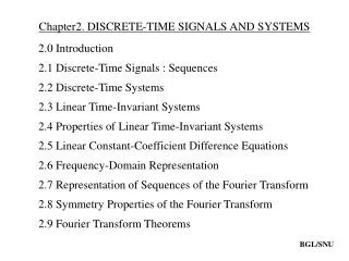
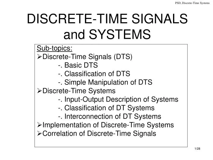
DISCRETE-TIME SIGNALS and SYSTEMS. Sub-topics: Discrete-Time Signals (DTS) -. Basic DTS -. Classification of DTS -. Simple Manipulation of DTS Discrete-Time Systems -. Input-Output Description of Systems -. Classification of DT Systems -. Interconnection of DT Systems

E N D
DISCRETE-TIME SIGNALS and SYSTEMS Sub-topics: Discrete-Time Signals (DTS) -. Basic DTS -. Classification of DTS -. Simple Manipulation of DTS Discrete-Time Systems -. Input-Output Description of Systems -. Classification of DT Systems -. Interconnection of DT Systems Implementation of Discrete-Time Systems Correlation of Discrete-Time Signals
Discrete-Time Signals • A DTS x(n) is a function of an independent variable that is integer
Some Representations of DTS • Functional representation • 2. Tabular representation • 3. Sequence representation
(n) 1 … … n u(n) 1 … … n Some Elementery DTS • The Unit Sample Sequence or Unit Impulse • The Unit Step Signal
ur(n) … … n • 3. The Unit Ramp Signal 4. The Exponential Signal x(n) = an,
Classification of DTS • Energy signals and power signals • Energy signal E can be finite and infinite. • If E is finite (0<E<∞), then x(n) is energy signal, P=0. • If E is infinite, then P can be finite or infinite. • If P is finite and P0, then signal x(n) is called power signal. • Periodic signals and aperiodic signals x(n+N) = x(n), all n -> periodic (N = period) Otherwise is aperiodic
Symmetric (even) and anti-symmetric (odd) signals • x(-n) = x(n) • x(-n) = -x(n)
Manipulation of Discrete-Time Signals • Transformation of the independent variable (time) • A signal x(n) is shifted in time by replacing the independent variable n by n-k, where k is integer • Results: delay of the signal (k is positive) or an advance of the signal (k is negative) • Folding or Reflection of signal (n becomes –n about the time origin n = 0)
Downsampling process • Replacing n by n, where is integer
Addition, multiplication, and scaling of sequences • Amplitude scaling: y(n) = A x(n) ; -∞<n<∞ ; A is a constant • The sum of two signals: y(n) = x1(n) + x2(n); -∞<n<∞ • The product of two signals: y(n) = x1(n).x2(n); -∞<n<∞ • Discrete-Time Systems • y(n) [x(n)] Accumulator: the system computes the current value of the input to the previous output value
x1(n) y(n) = x(n+1) x(n) Z y(n) = x1(n) + x2(n) + x2(n) a y(n) = a x(n) x(n) y(n) = x1(n) x2(n) x1(n) x x2(n) y(n) = x(n-1) x(n) Z-1 • Block Diagram Representation of Discrete-Time Systems • An Adder: memoryless process • A constant multiplier: memoryless process • A signal multiplier: memoryless process • A unit delay element: Z-1 is not memoryless • A unit advance element: not memoryless
Classification of Discrete-Time Systems • Static versus dynamic systems • Static • It is memoryless • Its output at any instant n depends at most on the input sample at the same time, but not on past or future samples of the input. • Dynamic • It has a memory • Its output at time n is completely determined by the input samples in the interval from n-k to n(k0), the system is said to have memory of duration k. • If k=0, the system is static • If 0<k<, the system is said to have finite memory • If k = , the system is said to have infinite memory • Time-invariant versus time-variant systems • Linear versus nonlinear systems • Causal versus non-causal systems • Stable versus unstable systems
Static vs Dynamic systems • Time-invariant versus time-variant systems • TI systems or shift invariant • If its input-output characteristics do not change with time Theorem. A relaxed system is time invariant if and only if:
Time-variant • If the output y(n,k) y(n-k), even for one value of k.
Linear vs non-linear systems • A linear system is a system that satisfies the superposition principle • Otherwise non-linear systems Theorem. A system is linear if and only if • E.g. Linear systems: • y1(n) = x1(n2) dan y2(n) = x2(n2), with superposition principle: • y3(n) = [a1x1(n) + a2x2(n)] = a1x1(n2) + a2x2(n2), then • a1y1(n) + a2y2(n) = a1x1(n2) + a2x2(n2) • e.g. Non-Linear Systems: • y(n) = ex(n), jika x(n) = 0 then y(n) = 1.
Causal versus non-causal systems • Causal system • If the output of the system at any time n [i.e., y(n)] depends only on present and past inputs [i.e., x(n), x(n-1), x(n-2), …] • Non-causal systems • Its output depends not only on present and past inputs but also on future inputs • Stable versus unstable systems • Stable system • Theorem. An arbitrary relaxed system is said to be bounded input – bounded output (BIBO) stable if and only if every bounded input produces a bounded output. • Bounded: existed finite numbers • x(n), y(n) = input, output • Mx, My = finite number • h(n) = impuls respon |x(n)| Mx < ∞ ; |y(n)| My < ∞ ;
y1(n) x(n) y(n) 1 2 c • Unstable system • If, for some bounded input sequence x(n), the output is unbounded (infinite) • Interconnection of Discrete-Time Systems • Cascade interconnection/series • Parallel interconnection y1(n) = 1 [x(n)] y(n) = 2 [y1(n)] = 2 [1 [x(n)]] c2 1 y(n) = c [x(n)] Cascade interconnection
p y1(n) 1 x(n) y3(n) + 2 y2(n) • Parallel: • y3(n) = y1(n) + y2(n) = 1[x(n)] + 2[x(n)] = (1+ 2)[x(n)] = p[x(n)] • p = (1+ 2) • Analysis of Discrete-Time Linear Time-Invariant Systems: • Convolution technique • It involves input, output signals, and impuls respons. • Math. Techniques that combine two signals to create a new signal
a. Low-Pass Filter (LPF) • Examples of application of convolution b. High-Pass Filter (HPF)
In math. Expression: • y(n): output signal, x(n): input signal and h(n): impuls respon • Convolution can be done in 4 steps: • Folding: Fold h(k) to k=0 to get h(-k) • Shifting: shift h(-k) by n0 to the right (left) if n0 is positive (negative) to get h(n0 – k) • Multiplication: multiply x(k) to h(n0 – k) to obtain the sequence vno(k) x(k)h(no – k). • Summation: Sum the sequence vno(k) to obtain the output value at n = no.
Convolution: vo(k) x(k)h(-k)
x(n) y(n) h(n) y(n) h(n) x(n) • Property of convolution and the interconnection of LTI systems • Commutative Law: x(n) * h(n) = h(n) * x(n) • Associative Law: [x(n) * h1(n)] * h2(n) = x(n) * [h1(n) * h2(n)] • Distributive Law:x(n) * [h1(n) + h2(n)] = x(n) * h1(n) + x(n) * h2(n) • Commutative Law • Associative Law
Distributive Law • Interconnection of LTI systems • Direct-Form I and Direct-Form II. • Direct-Form I uses delay (memory) element seperately between sample of input signal and output signal. • Direct-Form II, both input and output signal use the same delay elements. Hence Direct-Form II is more eficient. y(n) = -a1 y(n-1) + bo x(n) + b1 x(n-1) v(n) = bo x(n) + b1 x(n-1) (non-recursive) ; y(n) = -a1 y(n-1) + v(n) (Fig. b) or w(n) = -a1 w(n-1) + x(n) y(n) = bo w(n) + b1 w(n - 1)
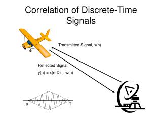
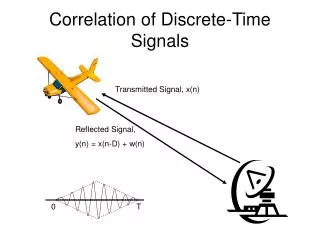
Correlation technique in Discrete Systems • It is used to measure the degree to which the two signals are similar and thus to extract some information that depends to a large extent on the application • Cross-correlation: correlation technique on two different signals • Autocorrelation: on two same signals The relationship between transmitted signal and reflected signal [ x(n) and y(n)] y(n) = x(n – D) + w(n) = attenuation factor in the round-trip transmission D = delay round-trip w(n) = additive noise system
Crosscorrelation • Autocorrelation • Correlation technique of sequences: • a. Shifting of any one of sequences. • b. Multiplication of two sequences. • c. Summing of all values of n.