Download
1 / 32
350 likes | 479 Views
Bitmapped Images. Chapter 5 Nigel Chapman & Jenny Chapman. 118. Bitmapped Images. Also known as raster graphics Record a value for every pixel in the image Often created from an external source Scanner, digital camera, …

E N D
Bitmapped Images • Chapter 5 • Nigel Chapman & Jenny Chapman
118 Bitmapped Images • Also known as raster graphics • Record a value for every pixel in the image • Often created from an external source • Scanner, digital camera, … • Painting programs allow direct creation of images with analogues of natural media, brushes, …
Most Popular Formats • Dozens of Formats, but 3 that matter • GIF – Graphics Interchange Format • Developed by CompuServe 1987 • JPEG - Joint Photographic Experts Group • Standard 1992 • PNG – Portable Network Graphics • 1996
GIF (.gif) • Maximum Colors: 8-bit 256 • Great for • Icons, Logos, and Line Art • Basic graphics • Flat Colors • First format supported by browsers • RLE: Run length encoding (Lossless Compression) LZ77 Algorithm.
JPEG (.jpg) • Maximum Colors: 24-bit 16.7 million • Great for • Hi-resolution Photographs • Images with subtle color graduation • Variation of RLE: Compresses groups of pixels into a single unit (Lossy Compression)
PNG (.png) • Maximum Colors: 24-bit 16.7 million • Great for • Mixed images: Photos with graphics • Photos with transparency • Developed specifically for the web. • Lossless compression • Variable transparency • Can store vector and object info for editing
PNG Story • In the early days of the web… • There were few graphics tools that supported PNG format • People forgot about it • PNG was completely forgotten • Not supported by many browsers • Thus, no proliferation of PNG files.
PNG Story • Lossless compression (like GIFs) but superior colors 24-bit OR 8-bit. • PNG much better for photographic images than GIF • Better compression for flat color graphics compared to JPEG • PNG much better for line art, logos, etc than JPEG • Plus, support for layers and vector data.
PNG should replace GIFwith one exception • GIF excels at compressing flat color images • But so does 8-bit PNG • 8-bit PNG format supports variable transparency; • GIF only supports flat transparency • But, GIF support embedded animation • PNG has no animated format
PNG will not replace JPG • JPG excels at compressing photo realistic images (hi-res 3200+ X 2400+) • 24-bit PNG is good but not as good • JPG is not good at flat color compression • PNG handles flat color much better • Overall, JPG might be better for very large photos. • PNG is certainly better for mixed images and medium to low resolution.
118–119 Device Resolution • Printers, scanners: specify as dots per unit length, often dots per inch (dpi) • Desktop printer 600dpi, typesetter 1270dpi, scanner 300–3600dpi,… • Video, monitors: specify as pixel dimensions • PAL TV 768x576px, • 17” CRT monitor 1024x768px • 19”-20” LCD monitor 1280x1024px • dpi depends on physical size of screen
Device Resolution • What is the best resolution display you can buy for under $3000?
120 Image Resolution • Array of pixels has pixel dimensions, but no physical dimensions • By default, displayed size depends on resolution (dpi) of output device • physical dimension = pixel dimension/resolution • Can store image resolution (ppi) in image file to maintain image's original size • Scale by device resolution/image resolution
120–122 Changing Resolution • If image resolution < output device resolution, must interpolate extra pixels • Always leads to loss of quality • If image resolution > output device resolution, must downsample (discard pixels) • Quality will often be better than that of an image at device resolution (uses more information) • Image sampled at a higher resolution than that of intended output device is oversampled
122–123 Compression • Image files may be too big for network transmission, even at low resolutions • Use more sophisticated data representation or discard information to reduce data size • Effectiveness of compression will depend on actual image data • For any compression scheme, there will always be some data for which 'compressed' version is actually bigger than the original
122–125 Lossless Compression • Always possible to decompress compressed data and obtain an exact copy of the original uncompressed data • Data is just more efficiently arranged, none is discarded • Run-length encoding (RLE) • Huffmann coding • Dictionary-based schemes – LZ77, LZ78, LZW (LZW used in GIF, licence fee charged)
125–126 JPEG Compression • Lossy technique, well suited to photographs, images with fine detail and continuous tones • Consider image as a spatially varying signal that can be analysed in the frequency domain • Experimental fact: people do not perceive the effect of high frequencies in images very accurately • Hence, high frequency information can be discarded without perceptible loss of quality
125–127 DCT • Discrete Cosine Transform • Similar to Fourier Transform, analyses a signal into its frequency components • Takes array of pixel values, produces an array of coefficients of frequency components in the image • Computationally expensive process – time proportional to square of number of pixels • Apply to 8x8 blocks of pixels
127 JPEG – Quantization • Applying DCT does not reduce data size • Array of coefficients is same size as array of pixels • Allows information about high frequency components to be identified and discarded • Use fewer bits (distinguish fewer different values) for higher frequency components • Number of levels for each frequency coefficient may be specified separately in a quantization matrix
127 JPEG – Encoding • After quantization, there will be many zero coefficients • Use RLE on zig-zag sequence (maximizes runs) • Use Huffman coding of other coefficients (best use of available bits)
128 JPEG – Decompression • Expand runs of zeros and decompress Huffman-encoded coefficients to reconstruct array of frequency coefficients • Use Inverse Discrete Cosine Transform to take data back from frequency to spatial domain • Data discarded in quantization step of compression procedure cannot be recovered • Reconstructed image is an approximation (usually very good) to the original image
129 Compression Artifacts • If use low quality setting (i.e. coarser quantization), boundaries between 8x8 blocks become visible • If image has sharp edges these become blurred • Rarely a problem with photographic images, but especially bad with text • Better to use good lossless method with text or computer-generated images
130 Image Manipulation • Many useful operations described by analogy with darkroom techniques for altering photos • Correct deficiencies in image • Remove 'red-eye', enhance contrast,… • Create artificial effects • Filters: stylize, distort,… • Geometrical transformations • Scale (change resolution), rotate,…
131–132 Selection • No distinct objects (contrast vector graphics) • Selection tools define an area of pixels • Draw selection (pen tool, lasso) • Select regular shape (rectangular, elliptical, 1px marquee tools) • Select on basis of colour/edges (magic wand, magnetic lasso) • Adjustments &c restricted to selected area
132–135 Masks • Area not selected is protected, as if masked by stencil • Can represent on/off mask as array of 1 bit per pixel (b/w image) • Generalize to greyscale image (semi-transparent mask) – alpha channel • Feathered and anti-aliased selections • Use as layer mask to modify layer compositing
136 Pixel Point Processing • Compute new value for pixel from its old value • p' = f(p), f is a mapping function • In greyscale images, ppp alters brightness and contrast • Compensate for poor exposure, bad lighting, bring out detail • Use with mask to adjust parts of image (e.g. shadows and highlights)
136–139 Adjustments in Photoshop • Brightness and contrast sliders • Adjust slope and intercept of linear f • Levels dialogue • Adjust endpoints by setting white and black levels • Use image histogram to choose values visually • Curves dialogue • Interactively adjust shape of graph of f
139–142 Pixel Group Processing • Compute new value for pixel from its old value and the values of surrounding pixels • Filtering operations • Compute weighted average of pixel values • Array of weights k/a convolution mask • Pixels used in convolution k/a convolution kernel • Computationally intensive process
142–144 Blurring • Classic simple blur • Convolution mask with equal weights • Unnatural effect • Gaussian blur • Convolution mask with coefficients falling off gradually (Gaussian bell curve) • More gentle, can set amount and radius
144–147 Sharpening • Low frequency filter • 3x3 convolution mask coefficients all equal to -1, except centre = 9 • Produces harsh edges • Unsharp masking • Copy image, apply Gaussian blur to copy, subtract it from original • Enhances image features
148–150 Geometrical Transformations • Scaling, rotation, etc. • Simple operations in vector graphics • Requires each pixel to be transformed in bitmapped image • Transformations may 'send pixels into gaps' • i.e. interpolation is required • Equivalent to reconstruction & resampling; tends to degrade image quality
150–151 Interpolation • Nearest neighbour • Use value of pixel whose centre is closest in the original image to real coordinates of ideal interpolated pixel • Bilinear interpolation • Use value of all four adjacent pixels, weighted by intersection with target pixel • Bicubic interpolation • Use values of all four adjacent pixels, weighted using cubic splines