Download
1 / 19
190 likes | 344 Views
Images. Course web page: vision.cis.udel.edu/cv. March 3, 2003 Lecture 8. Announcements . Homework is due tonight by midnight (LaTeX broken in Smith 040) Read about convolution in Chapter 7-7.2, 7.5-7.7 of Forsyth and Ponce for Wednesday. Outline.

E N D
Images Course web page: vision.cis.udel.edu/cv March 3, 2003 Lecture 8
Announcements • Homework is due tonight by midnight (LaTeX broken in Smith 040) • Read about convolution in Chapter 7-7.2, 7.5-7.7 of Forsyth and Ponce for Wednesday
Outline • Digitization will be discussed in the camera lecture (#16) • Image types, basic operations in Matlab • Binary images • Image comparison • Texture mapping
Matlab Image Types • Note: Although we write I(x, y), remember that Matlab uses I(r, c) • Intensity: mxn matrix. Can be: • uint8: Unsigned 8-bit integer—i.e., in the range [0…255] • double: Real number in range [0…1] • True color: mxnx3 • Basically, stacked red, green, and blue intensity images (aka channels) • Binary: Values are 0 or 1, type logical
Image Type Conversions • Many functions work on just one channel • Run on each channel independently • Convert from color grayscale weighting each channel by perceptual importance (rgb2gray) • Some operations want the pixels to be real-valued • Type conversion: I2 = double(I1)
Image Arithmetic • Just like matrices, we can do pixelwise arithmetic on images • Some useful operations • Differencing: Measure of similarity • Averaging: Blend separate images or smooth a single one over time • Thresholding: Apply function to each pixel, test value • In Matlab: imadd, imsubtract, imcomplement, imlincomb, etc. • Beware of truncation • Can do all of these with matrix operations if you pay attention to types and truncation
Thresholding • Grayscale Binary: Choose threshold based on histogram of image intensities (Matlab: imhist)
Example: Image Histograms courtesy of MathWorks
Derived Images: Color Similarity as Chrominance Distance • Distance to red in YIQ space (rgb2ntsc) • Can threshold on this
Connected Components • Uniquely label each n-connected region in binary image • 4- and 8-connectedness • Matlab: bwfill, bwselect
Example: Connected Components courtesy of HIPR
Binary Operations • Dilation, erosion (Matlab: imdilate, imerode) • Dilation: All 0’s next to a 1 1 (Enlarge foreground) • Erosion: All 1’s next to a 0 0 (Enlarge background) courtesy of Reindeer Graphics Original Eroded Dilated
Moments: Region Statistics • Zeroth-order: Size/area • First-order: Position (centroid) • Second-order: Orientation
Geometric Image Comparison: SSD • Given a template image IT and an image I, how to quantify the similarity between them? • Vector difference: Sum of squared differences (SSD)
Correlation for Template Matching • Note that SSD formula can be written: • When the last term is big, the mismatch is small—the dot product measures correlation: • By normalizing by the vectors’ lengths, we are measuring the angle between them
Normalized Cross-Correlation • Shift template image over search image, measuring normalized correlation at each point • Local maxima indicate template matches • Matlab: normxcorr2 from Jain, Kasturi, & Schunck
Statistical Image Comparison:Color Histograms • Steps • Histogram RGB/HSI triplets over two images to be compared • Normalize each histogram by respective total number of pixels to get frequencies • Similarity is Euclidean distance between color frequency vectors • Insensitive to geometric changes, including different-sized images • Matlab: imhist, hist
Image Transformations • Geometric: Compute new pixel locations • Rotate • Scale • Undistort (e.g., radial distortion from lens) • Photometric: How to compute new pixel values when non-integral • Nearest neighbor: Value of closest pixel • Bilinear interpolation (2 x 2 neighborhood) • Bicubic interpolation (4 x 4)
Vertical blend Horizontal blend Bilinear Interpolation • Idea: Blend four pixel values surrounding source, weighted by nearness