Download
1 / 20
200 likes | 291 Views
AMS 691 Special Topics in Applied Mathematics Review of Fluid Equations. James Glimm Department of Applied Mathematics and Statistics, Stony Brook University Brookhaven National Laboratory. Review of Equations of Fluid Flow.

E N D
AMS 691Special Topics in Applied MathematicsReview of Fluid Equations James Glimm Department of Applied Mathematics and Statistics, Stony Brook University Brookhaven National Laboratory
Review of Equations of Fluid Flow Reference: Chorin-Marsden. Also Landau-Lifshitz is a good reference We assume basic laws of Newtonian physics, applied to continuous rather than to discrete particle systems.
Thermodynamics p = pressure = density; V = 1/ = specific volume T = temperature s = entropy w = enthalpy = internal energy Any two are independent. Any third is a function of these two. P = p(s, ) First law of thermodynamics:
Euler Equations for Compressible Isentropic Flow If flow is not isentropic, we need one more equation for conservation of energy. For gamma law gas, Reference: Courant-Friedrichs
Wave curves and the Riemann Problem We have defined three types of wave curves: forward (right moving) shock or rarefaction waves contacts backward (left moving) shock or rarefaction waves In 1D, the number of variables (dimension of state space) is 3: Conserved density, momentum, energy. Also called the primitive variables Thus there is one type of wave curve for each dimension. If we compose the three wave curves, we sweep out a 3D region in state space. To realize this construction, we pick the three waves in A definite order, starting from the right, with the fastest first. This is the order listed above. Thus any sequence of waves (taken along a wave curve from a given starting point) defines a solution of conservation laws, joining starting state to final state. It is a Riemann solution, of the Riemann problem with right state = start, left state = finish.
Riemann problems In the wave curve picture, we see that a rarefaction is a kind of negative shock wave, in that it moves in the opposite direction. It is also close but not identical to the Hugoniot curve followed in the “wrong” direction. Similarly, the Hugoniot curve is close but not identical to the rarefaction curve (adiabat) defining a rarefaction in the “wrong” direction. For most equations of state (EOS), this wave curve map, from start to final state covers all of the state space. In other words, for most EOS, and any pair of left and right states, there is a (unique) solution of the Riemann problem with this data, formed of three waves, that is defined by the three wave curves. These ideas are at the basis of a number of numerical schemes for conservation laws. See the book by Levesque.
Solving Riemann Problems The waves at the right/left are shocks/rarefactions; the one in the center is a contact. Across the contact, pressure and (normal) velocity are continuous. Let u*, P* denote this common value on the two sides of the contact.