Download

1 / 21
360 likes | 865 Views
Fluid equations, magnetohydrodynamics. Multi-fluid theory Equation of state Single-fluid theory Generalised Ohm‘s law Magnetic tension and plasma beta Stationarity and equilibria Validity of magnetohydrodynamics. Multi-fluid theory.

E N D
Fluid equations, magnetohydrodynamics • Multi-fluid theory • Equation of state • Single-fluid theory • Generalised Ohm‘s law • Magnetic tension and plasma beta • Stationarity and equilibria • Validity of magnetohydrodynamics
Multi-fluid theory • Full plasma description in terms of particle distribution functions (VDFs), fs(v,x,t), for species, s. • For slow large-scale variations, a description in terms of moments is usually sufficient -> multi-fluid (density, velocity and temperature) description • Magnetohydrodynamics is the single-fluid theory of electrically charged mixed fluids subject to the presence of external and internal magnetic fields. • Fluid theory is looking for evolution equations for the basic macroscopic moments, i.e. number density, ns(x,t), velocity, vs(x,t), pressure tensor, Ps(x,t), and kinetic temperature, Ts(x,t). For a two fluid plasma consisting of electrons and ions, we have s=e,i.
Continuity equation Evolution equation of moments are obtained by taking the corresponding moments of the Vlasov equation: Taking the zeroth moment yields for the first term: In the second term, the velocity integration and spatial differentiation can be interchanged which yields a divergence: In the force term, a partial integration leads to a term, which does not contribute. Collecting terms gives:
Momentum equation I The evolution equation for the momentum is obtained by taking the first moment of the Vlasov equation: Since the phase space coordinate v does not depend on time, the first term yields the time derivative of the flux density: In the second term, velocity integration and spatial differentiation can be exchanged, and v(v·x) = x·(vv) be used. We decompose the dyadic as: In the second term, the resulting four contributions can be combined to give:
Momentum equation II In the third term, a partial integration with respect to the velocity gradient operator v gives the remaining integral: We can now add up all terms and obtain the final result: This momentum density conservation equation for species s resembles in parts the one of conventional hydrodynamics, the Navier-Stokes equation. Yet, in a plasma for each species the Lorentz force appears in addition, coupling the plasma motion (via current and charge densities) to Maxwell‘s equation and also the various components (electrons and ions) among themselves.
Energy equation The equations of motion do not close, because at any order a new moment of the next higher order appears (closure problem), leading to a chain of equations. In the momentum equation the pressure tensor, Ps, is required, which can be obtained from taking the seond-order moment of Vlasov‘s equation. The results become complicated. Often only the trace of Ps, the isotropic pressure, ps, is considered, and the traceless part, P's ,the stress tensor is separated, which describes for example the shear stresses. The full energy (temperature, heat transfer) equation reads: The sources or sinks on the right hand side are related to heat conduction, qs, or mechanical stress, P's.
Equation of state I A truncation of the equation hierarchy can be achieved by assuming an equation of state, depending on the form of the pressure tensor. If it is isotropic, Ps = ps1, with the unit dyade, 1, and ideal gas equation, ps= nskBTs, then we have a diagonal matrix: • Isothermal plasma: Ts = const • Adiabatic plasma: Ts = Ts0 (ns/ns0)-1, with the adiabatic index = cP/cV = 5/3 for a mono-atomic gas.
Equation of state II Due to strong magnetization, the plasma pressure is often anisotropic, yet still gyrotropic, which implies the form: with a different pressure (temperature) parallel and perpendicular to the magnetic field. Then one has two energy equations, which yield (without sinks and sources) the double-adiabatic equations of state: • T B -> perpendicular heating in increasing field • T|| (n/B)2 -> parallel cooling in declining density
One-fluid theory Consider simplest possible plasma of fully ionized hydrogen with electrons with mass me and charge qe = -e, and ions with mass mi and charge qi = e. We define charge and current density by: Usually quasineutrality applies, ne= ni, and space charges vanish, = 0, but the plasma carries a finite current, i.e. we still need an equation for j. We introduce the mean mass, density and velocity in the single-fluid description as
One-fluid momentum equation Constructing the equation of motion is more difficult because of the nonlinear advection terms, nsvsvs. To be general, we include some friction term, R = Rie= -Rie, because of momentum conservation requires the two terms to be of opposite sign. The equation of motion is obtained by adding these two equations and exploiting the definitions of , m, n, v and j. When multiplying the first by me and the second by mi and adding up we obtain: Here we introduced the total pressure tensor, P = Pe + Pi. In the nonlinear parts of the advection term we can neglect the light electrons entirely.
Magnetohydrodynamics (MHD) With these approximations, which are good for many quasineutral space plasmas, we have the MHD momentum equation, in which the space charge (electric field) term is also mostly disregarded. Note that to close the full set, an equation for the current density is needed. For negligable displacement currents, we simply use Ampere‘s law in magnetohydrodynamics and B as a dynamic variable, and replace then the Lorentz force density by:
Generalized Ohm‘s law I The evolution equation for the current density, j, is derived by use of the electron equation of motion and called generalized Ohm‘s law. It results from a subtraction of the ion and electron equation of motion. The nonlinear advection terms cancel in lowest order. The result is: The right hand sides still contain the individual densities, masses and speeds, which can be eliminated by using that me/mi << 1, neni. Hence we obtain a simplified equation: Key features in single-fluid theory: Thermal effects on j enter only via, Pe, i.e. the electron pressure gradient modulates the current. The Lorentz force term contains the electric field as seen in the electron frame of reference.
Generalized Ohm‘s law II Omitting terms of the order of the small mass ratio, the fluid bulk velocity is, vi = v. Using this and the quasineutrality condition yields the electron velocity as: ve = v - j/ne. Finally, the collision term with frequency c can be assumed to be proportional to the velocity difference, and use of the resistivity, =mec/ne2, permits us to write: The resulting Ohm‘s law can then be written as: The right-hand side contains, in a plasma in addition to the resistive term, three new terms: electron pressure, Hall term, contribution of electron inertia to current flow. In an ideal plasma, =0, with no pressure gradient and slow current variations, the field is frozen to the electrons:
Magnetic tension The Lorentz force or Hall term introduces a new effect in a plasma which is specific for magnetohydrodynamics: magnetic tension, giving the conducting fluid stiffness. For slow variations Ampere‘s law can be used to derive: Applying some vector algebra (left as exercise) to the right hand side gives: The first term corresponds to a magnetic pressure, and the second is the divergence of the magnetic stress tensor: - BB/0
Plasma beta Starting from the MHD equation of motion for a plasma at rest in a steady quasineutral state, we obtain the simple force balance: which expresses magnetohydrostatic equilibrium, in which thermal pressure balances magnetic tension. If the particle pressure is nearly isotropic and the field uniform, this leads to the total pressure being constant: The ratio of these two terms is called the plasma beta:
Electrostatic equilibrium: Boltzmann‘s law Consider the stationary electron momentum equation with scalar pressure and without magnetic field. Setting the convective derivative to zero yields: The electric field can be represented by an electrostatic potential, E = -, and assume that the electrons are isothermal with pe = nekBTe, then we have and by integration the Boltzmann law, which relates the stationary electron density to the electric potential in an exponential way: Electrons react very sensitively to an electric field.
Diamagnetic drift Let us return to the s-component fluid equation under stationary conditions and with an anisotropic pressure tensor. The equations of motion then express the balance between the Lorentz forces and individual pressure gradients such that Taking the cross product with B/B2 and rearranging the terms, we obtain the stationary drift velocity of species s as follows: Diamagnetic current:
Neutral sheet current A typical example of a diamagnetic current is the neutral sheet in the magnetotail of the Earth, which divides the regions of inward (in the northern lobe) and outward magnetic fields. Parameters: temperature 1-10 keV, transverse field 1-5 nT, density 1 cm-3, thickness 1-2 RE, and very high plasma beta, = 100. The Harris model sheet is shown below. A simple analytical model field is given by a hyperbolic tangent function: Here BL is the lobe magnetic field, and LB its variation scale length.
Force-free magnetic fields A special equilibrium of ideal MHD (often used in case of the solar corona) occurs if the beta is low, such that the pressure gradient can be neglected. The stationary plasma becomes force free, if the Lorentz force vanishes: This condition is guaranteed if the current flows along the field and obeys: The proportionality factor L(x) is called lapse field. Ampère‘s law yields: By taking the divergence, one finds that L(x) is constant along any field line:
Requirements for the validity of MHD Variations must be large and slow, < gi and k < 1/rgi, which means fluid scales must be much larger than gyro-kinetic scales. Consider Ohm‘s law: Convection, Hall effect, thermoelectricity, polarization, resistivity gi /c /c Only in a strongly collisional plasma can the Hall term be dropped. In collisionless MHD the electrons are frozen to the field.