Download
1 / 17
170 likes | 315 Views
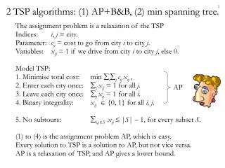
2 TSP algorithms: (1) AP+B&B, (2) min spanning tree. The assignment problem is a relaxation of the TSP Indices: i , j = city. Parameter: c ij = cost to go from city i to city j . Variables: x ij = 1 if we drive from city i to city j , else 0. Model TSP:

E N D
2 TSP algorithms: (1) AP+B&B, (2) min spanning tree. • The assignment problem is a relaxation of the TSP • Indices: i, j = city. • Parameter: cij= cost to go from city i to city j. • Variables: xij= 1 if we drive from city i to city j, else 0. • Model TSP: • 1. Minimise total cost: min ij cij xij, • 2. Enter each city once: i xij = 1 for all j. • 3. Leave each city once: j xij = 1 for all i. • 4. Binary integrality: xij {0, 1} for all i, j. • 5. No subtours: i,jS xij |S| – 1, for every subset S. • (1) to (4) is the assignment problem AP, which is easy. • Every solution to TSP is a solution to AP, but not vice versa. • AP is a relaxation of TSP, and AP gives a lower bound. AP
One way to break subtours: B&B • We can break subtours by adding constraints:x3,2 + x2,4 + x4,3 2. • After solving again, other subtours appear. • Instead, we can branch on a variable in the subtour:Create an assignment subproblem with x4,3 = 0. • This is a B&B algorithm specialised for the TSP. 3 3 1 1 4 4
Example, Winston (2003), pp. 530-534 • When we solve subproblem S1, we get subtours 1-2-5-1, 3-4-3. • In the optimal solution, either x3,4 = 0 or x4,3 = 0. • So let’s make 2 subproblems, S2 for x3,4=0, and S3 for x4,3=0.
With x3,4 = 0, we get 1-4-3-1 instead of 1-3-4-1. • We also have the subtour 2-5-2. • Let’s branch on x2,5=0 for S4. (To do list: S3 with x4,3 = 0.)
S4 gives a tour! 1-5-2-4-3-1 • So we have an upper bound of 668. • The optimum is 668 or less.
The complete B&B tree S1: ov=495, 1-2-5-1, 1-3-4-1. • At S4, we found a tour of length 668. • The tours at S5 and S6 are worse, so they are not optimal. • S7 has subtours, but more constraints cannot help 910, so we quit.So S4 gives the optimal tour, 1-5-2-4-3-1. • So we can solve the TSP with B&B, with AP as the subproblem.Each AP subproblem was a relaxation. Are there other relaxations? x3,4 = 0 x4,3 = 0 S2: ov=652, 1-4-3-1, 2-5-2 S3: ov=652 1-3-4-1, 2-5-2 x5,2 = 0 x2,5 = 0 x2,5 = 0 x5,2 = 0 S4: ov=668, 1-5-2-4-3-1. S5: ov=704, 1-4-3-2-5-1. S6: ov= 704, 1-5-2-3-4-1 S7: ov=910, 1-3-1, 2-5-4-2
Another TSP relaxation: the one-tree • First some definitions. • Tree: connected graph with no loops. • One-tree: a tree plus one loop. Hey! This one tree is a tour!Every tour is a one-tree,but not every one-tree is a tour.
The minimum spanning tree problem (MST) • MST: Find the shortest tree that connects all the dots. • Not a good one! • This is much better: • Many applications: telecommunications, road networks. • How do we find the minimum spanning tree? 2 ways, Prim’s algorithm or Kruskal’s algorithm.
Prim’s algorithmFind the closest node that doesn’t make a loop • Step 0. Sort all the arcs in increasing order.The tree is empty except for node 1. • Step 1. Find the smallest arc i, j or j, i that connects to any node i in the tree.If arc i, j makes a loop, skip it. Else add it to the tree. • Step 2. If all the nodes are connected, you’re done.Else, go back to Step 1. • See http://www-b2.is.tokushima-u.ac.jp/~ikeda/suuri/dijkstra/PrimApp.shtml?demo7
Kruskal’s algorithm:Find the smallest arc that doesn’t make a loop • Step 0. Sort all the arcs in increasing order.The tree is empty. • Step 1. Find the shortest arc on the list.If it makes a loop, delete it. Else add it to the tree. • Step 2. If all the nodes are connected, you’re done.Else, go back to Step 1. • See http://www-b2.is.tokushima-u.ac.jp/~ikeda/suuri/kruskal/KruskalApp.shtml?demo5
Demo of each algorithm 5 • From To Length Prim Kruskal • 7 8 5.1 6 1 • 6 8 14.3 7 2 • 6 7 14.5 - - • 2 4 17.1 2 3 • 2 3 25.8 3 4 • 4 9 28.8 4 5 • 4 8 29.9 5 6 • 8 9 30.2 - - • 4 7 31.2 - - • 3 4 31.9 - - • 5 7 32.5 8 7 • 7 9 35.0 - - • 2 9 36.4 - - • 5 6 37.0 - - • 5 8 37.6 - - • 6 9 39.5 - - • 1 2 41.0 1 8 • 4 6 44.2 - - • 2 8 46.6 - - • 1 9 47.7 - - • 2 7 48.2 - - Prim – closest node 3 7 4 6 2 8 9 5 Kruskal – smallest arc 1 3 7 4 6 2 8 9 Exercise: Label the arcs in the order added. 1
5 3 7 4 6 2 8 9 1 We can make an MST, how about a 1-tree? • To make a minimum 1-tree: • Step 1. Find the MST of all nodes except node 1. • Step 2. Add the 2 smallest arcs that connect to node 1. • This is easy work.You can do it for 100 cities in a few minutes by hand.
The 1-tree length is a lower bound on the TSP • But not a very good one, typically only 63% of the optimum.Our example is only 67% of the optimum. • What is wrong with the minimum 1-tree?In the TSP, every node has 2 arcs, one in and one out.In the min 1-tree, some nodes have 1 arc, some have more than 2. • We can improve the lower bound as follows:Solve the 1-tree problem, but add a penalty to each arcthat comes into a node with the wrong number of arcs. length=194.5 length=287.1 5 5 3 3 7 7 4 4 6 6 2 2 8 8 9 9 1 1
Recall the symmetric TSP formulation • 1. Minimise total cost: min ij>i cij xij, • 2. Enter each city once: j<i xji+ j>i xij = 2 for all i. • 3. Subtour breaking: i,jS xij |S| – 1, for each subset S. • 4. Binary integrality: xij {0, 1} for all i, j. • Subtours (set 3) are not the problem with the min 1-tree. • Entering each city (set 2) once is the problem with the min 1-tree. • Another way to put the TSP: • 1. Minimise total cost: min ij>i cij xij, • 2. Enter each city once: j<i xji+ j>i xij = 2 for all i. (λi) • 3. Must be a 1-tree: x T, where T is the set of all 1-trees. • Let’s relax set 2, as for a Dantzig-Wolfe subproblem: • 1. Minimise total cost: min ij>i cij xij + iλi(j<i xji+ j>i xij– 2) = min ij>i (cij + λi + λj)xij – 2i λi • 3. Must be a 1-tree: x T, where T is the set of all 1-trees.
TSP lower bound with subgradient optimisation • Step 0. Set λi = 0. (Cleverer to start with AP’s dual prices.) • Pick a jump size tk between 0.5 and 2. • Set a small ending tolerance > 0. • Set k = 1. • Step 1. Solve the min 1-tree problem. 1-tree(λik): min ij>i cij xij + iλi(j<i xji+ j>i xij– 2) x T, where T is the set of all 1-trees. • Step 2. Let dik be number of arcs coming into node i at iteration k. • If node i is good, dik = 2, keep the penalty:set λik+1 = λik. • If node i is bad, dik ≠ 2, change the penalty: set λik+1 = λik + tk (dik − 2). • Step 3. If |k+1 – k| < , stop. Else set tk+1 = tk ·0.9, set k = k+1 and go to Step 1. Excellent animated examples:http://itp.nat.uni-magdeburg.de /~mertens/TSP/
5 3 7 4 6 2 8 9 1 Still no promises, but not bad. • Subgradient opt gets a better lower bound than plain 1-tree, often 99%. • But it can take a long time. No guarantee we get an optimum. • Example: Starting with step size=5, then 1, then 0.5, we getλk = {-41.0, -12.5, -27.5, -19.0, -45.5, -27.5, -20.0, -19.0, -22.0}, • and the optimal tour: • Why are the prices negative? • Not hard to do in AMPL, even possible with Excel & Visual Basic. • Another B&B scheme: use 1-trees for subproblems.Branch on arcs that go into nodes with degree ≠ 2.
The 1-tree gives 2 lower bounds – bad & good • At the beginning, with all λi=0,we get a bad lower bound. This is just the smallest 1-tree. • During subgradient optimisation,we can say nothing about bounds. • At the end of subgradient optimisation, with the optimalλ’s,we get a good lower bound. • The lower bound is the penalised length,not the ordinary length of the 1-tree. • The ordinary (unpenalised) length of the optimised 1-treecould be longer than the optimal tour! • If all nodes have degree 2, penalised length = ordinary length,and we have the optimal tour. • Ref: Held, M., & Karp, R., “The Traveling-Salesman Problem and Minimum Spanning Trees” Ops Research, v.18, n.6, Nov-Dec 1970. • Next: more on subtours & trees. We’ll also cover this in tutorial.