Download
1 / 10
350 likes | 1.3k Views
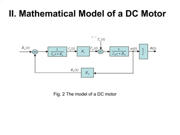
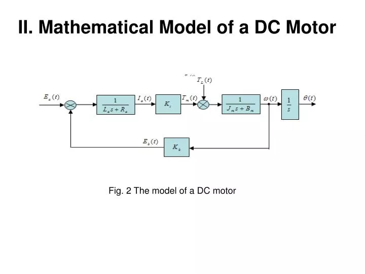
II. Mathematical Model of a DC Motor. Fig. 2 The model of a DC motor. III. Sliding Mode Controller. The sliding mode control schemes have been widely developed over several decades of years.

E N D
II. Mathematical Model of a DC Motor Fig. 2 The model of a DC motor
III. Sliding Mode Controller • The sliding mode control schemes have been widely developed over several decades of years. • Essentially, the SMC uses discontinuous control action to drive state trajectories toward a specific hyperplane in the state space, and to maintain the armature or the control of the field. • Easy controlling and cheapness of the circuit drive of the DC motors comparing to AC motors has lead to be chosen by the consumers and industries. • DC motors are done mainly controls through the control of the state trajectories sliding on specific hyper plane until the origin of the state space is reached.
III. Sliding Mode Controller • In an SMC system [6], the control commands are adequately designed such that the states will move towards the desired sliding plane. • Once the states reach the sliding surface, the system is said to be in sliding mode. • During the sliding mode, the system possesses some invariance properties, such as robustness, order reduction and disturbance rejection. • The first step to design a sliding mode control is to determine the sliding hyperplane with desired dynamics of the corresponding sliding motion. • And the next step is to design the control input so that the state trajectories are driven and attracted toward the sliding hyperplane and then remained sliding on it for all subsequent time.
III. Sliding Mode Controller • In the following, the sliding mode control for continuous and discrete time system is reviewed. • A Sliding Mode Controller is a Variable Structure Controller (VSC). Basically, a VSC includes several different continuous functions that can map plant state to a control surface, and the switching among different functions is determined by plant state that is represented by a switching function. • Without lost of generality, consider the design of a sliding mode controller for the following second order system; u(t) is the input to the system. • The following is a possible choice of the structure of a sliding mode controller u is a control law:
III. Sliding Mode Controller • Control law: u = −k sgn( s) + ueq • Where is called equivalent control which is used whenthe system state is in the sliding mode; and ; N is the constant, N>0 . The k is a gainand it is the maximal value of the controller output. • The s iscalled switching function because the control actionswitches its sign on the two sides of the switching surface s = 0 . The s is defined as: • Where and , is the desired state. λ is a constant. sgn(s) is a sign function, which is defined as: (7)
III. Sliding Mode Controller • The control strategy adopted here will guarantee the system trajectories move toward and stay on the sliding surface s = 0 from any initial condition if the following condition meets: • Where η is a positive constant that guarantees the system trajectories hit the sliding surface in finite time. Using a sign function often causes chattering in practice. One solution is to introduce a boundary layer around the switch surface (7) • Where= −k*sat(s /φ) and constant factor φ defines the thickness of the boundary layer. The sat(s/φ) is a saturation function which is defined as:
Sliding mode control law Where: or and Where:
III. Sliding Mode Controller Fig.3 The sliding surface and the boundary.
IV. Fuzzy Controller • The tracking error and the change of the error are defined asand(or ds). And s is sliding surface in (7) by or s(k) = de(k) +λ*e(k) and ds(k) = s(k) – s(k-1); • Where: s(k) = de(k) +λ*e(k); • s(k-1 )=de(k-1) - λe(k-1); (13) • and de(k-1)=e(k-1)-e(k-2); (14) • s(k-1) and de(k-1) for calculating in the FSM in Fig.6 • and s, ds and uf are input and output variables of FC, respectively. The design procedure of the FC is as follows:
IV. Fuzzy Controller • (a) Take the s and ds as the input variables of the FC, and define their linguist variables as S and dS. The linguist value of S and dS are {A0, A1, A2, A3, A4, A5, A6} and {B0, B1, B2, B3, B4, B5, B6}, respectively. Each linguist value of S and and dS. The linguist value of S and dS are {A0, A1, A2, A3, A4, A5, A6} and {B0, B1, B2, B3, B4, B5, B6}, respectively. Each linguist value of S and dS is based on the symmetrical triangular membership function which is shown in Fig.4.