Download
1 / 69
710 likes | 1.15k Views
A Mathematical Model of Motion. CHAPTER 5 PHYSICS. 5.1 Graphing Motion in One Dimension. Interpret graphs of position versus time for a moving object to determine the velocity of the object Describe in words the information presented in graphs and draw graphs from descriptions of motion

E N D
A Mathematical Model of Motion CHAPTER 5 PHYSICS
5.1 Graphing Motion in One Dimension • Interpret graphs of position versus time for a moving object to determine the velocity of the object • Describe in words the information presented in graphs and draw graphs from descriptions of motion • Write equations that describe the position of an object moving at constant velocity
Parts of a Graph • X-axis • Y-axis • All axes must be labeled with appropriate units, and values.
5.1 Position vs. Time • The x-axis is always “time” • The y-axis is always “position” • The slope of the line indicates the velocity of the object. • Slope = (y2-y1)/(x2-x1) • d1-d0/t1-t0 • Δd/Δt
Uniform Motion • Uniform motion is defined as equal displacements occurring during successive equal time periods (sometimes called constant velocity) • Straight lines on position-time graphs mean uniform motion.
Given below is a diagram of a ball rolling along a table. Strobe pictures reveal the position of the object at regular intervals of time, in this case, once each 0.1 seconds. Notice that the ball covers an equal distance between flashes. Let's assume this distance equals 20 cm and display the ball's behavior on a graph plotting its x-position versus time.
The slope of this line would equal 20 cm divided by 0.1 sec or 200 cm/sec. This represents the ball's average velocity as it moves across the table. Since the ball is moving in a positive direction its velocity is positive. That is, the ball's velocity is a vector quantity possessing both magnitude (200 cm/sec) and direction (positive).
Steepness of slope on Position-Time graph • Slope is related to velocity • Steep slope = higher velocity • Shallow slope = less velocity
Different Position. Vs. Time graphs Accelerated Motion Uniform Motion Constant positive velocity (zero acceleration) Increasing positive velocity (positive acceleration) Constant negative velocity (zero acceleration) Decreasing negative velocity (positive acceleration)
Different Position. Vs. Time Changing slope means changing velocity!!!!!! Increasing negative slope = ?? Decreasing negative slope = ??
X B A t C A … Starts at home (origin) and goes forward slowly B … Not moving (position remains constant as time progresses) C … Turns around and goes in the other direction quickly, passing up home
During which intervals was he traveling in a positive direction? During which intervals was he traveling in a negative direction? During which interval was he resting in a negative location? During which interval was he resting in a positive location? During which two intervals did he travel at the same speed? A) 0 to 2 sec B) 2 to 5 sec C) 5 to 6 sec D)6 to 7 sec E) 7 to 9 sec F)9 to 11 sec
x C B t A D Graphing w/ Acceleration A … Start from rest south of home; increase speed gradually B … Pass home; gradually slow to a stop (still moving north) C … Turn around; gradually speed back up again heading south D … Continue heading south; gradually slow to a stop near the starting point
You try it….. • Using the Position-time graph given to you, write a one or two paragraph “story” that describes the motion illustrated. • You need to describe the specific motion for each of the steps (a-f) • You will be graded upon your ability to correctly describe the motion for each step.
x Tangent Lines t On a position vs. time graph:
x t Increasing & Decreasing Increasing Decreasing On a position vs. time graph: Increasing means moving forward (positive direction). Decreasing means moving backwards (negative direction).
x t Concavity On a position vs. time graph: Concave up means positive acceleration. Concave down means negative acceleration.
x t Special Points Q R P S
5.2 Graphing Velocity in One Dimension • Determine, from a graph of velocity versus time, the velocity of an object at a specific time • Interpret a v-t graph to find the time at which an object has a specific velocity • Calculate the displacement of an object from the area under a v-t graph
5.2 Velocity vs. Time • X-axis is the “time” • Y-axis is the “velocity” • Slope of the line = the acceleration
Velocity vs. Time • Horizontal lines = constant velocity • Sloped line = changing velocity • Steeper = greater change in velocity per second • Negative slope = deceleration
Acceleration vs. Time Time is on the x-axis • Acceleration is on the y-axis • Shows how acceleration changes over a period of time. • Often a horizontal line.
x t All 3 Graphs v t a t
Real life Note how the v graph is pointy and the a graph skips. In real life, the blue points would be smooth curves and the orange segments would be connected. In our class, however, we’ll only deal with constant acceleration. v t a t
Graph Practice Try making all three graphs for the following scenario: 1. Newberry starts out north of home. At time zero he’s driving a cement mixer south very fast at a constant speed. 2. He accidentally runs over an innocent moose crossing the road, so he slows to a stop to check on the poor moose. 3. He pauses for a while until he determines the moose is squashed flat and deader than a doornail. 4. Fleeing the scene of the crime, Newberry takes off again in the same direction, speeding up quickly. 5. When his conscience gets the better of him, he slows, turns around, and returns to the crash site.
Area Underneath v-t Graph • If you calculate the area underneath a v-t graph, you would multiply height X width. • Because height is actually velocity and width is actually time, area underneath the graph is equal to • Velocity X time or V·t
Remember that Velocity = Δd Δt • Rearranging, we get Δd = velocity X Δt • So….the area underneath a velocity-time graph is equal to the displacement during that time period.
x “positive area” v t t “negative area” Area Note that, here, the areas are about equal, so even though a significant distance may have been covered, the displacement is about zero, meaning the stopping point was near the starting point. The position graph shows this as well.
Velocity vs. Time • The area under a velocity time graph indicates the displacement during that time period. • Remember that the slope of the line indicates the acceleration. • The smaller the time units the more “instantaneous” is the acceleration at that particular time. • If velocity is not uniform, or is changing, the acceleration will be changing, and cannot be determined “for an instant”, so you can only find average acceleration
5.3 Acceleration • Determine from the curves on a velocity-time graph both the constant and instantaneous acceleration • Determine the sign of acceleration using a v-t graph and a motion diagram • Calculate the velocity and the displacement of an object undergoing constant acceleration
5.3 Acceleration • Like speed or velocity, acceleration is a rate of change, defined as the rate of change of velocity • Average Acceleration = change in velocity Elapsed time Units of acceleration?
Finally… • This equation is to be used to find (final) velocity of an accelerating object. You can use it if there is or is not a beginning velocity
Displacement under Constant Acceleration • Remember that displacement under constant velocity was Δd = vt or d1 = d0 + vt • With acceleration, there is no one single instantaneous v to use, but we could use an average velocity of an accelerating object.
Average velocity of an accelerating object would simply be ½ of sum of beginning and ending velocities Average velocity of an accelerating object V = ½ (v0 + v1)
So……. Key equation
Some other equations 2 This equation is to be used to findfinalposition when there is an initial velocity, but velocity at time t1 is not known.
2 2 2 2 2
Practical Application Velocity/Position/Time equations • Calculation of arrival times/schedules of aircraft/trains (including vectors) • GPS technology (arrival time of signal/distance to satellite) • Military targeting/delivery • Calculation of Mass movement (glaciers/faults) • Ultrasound (speed of sound) (babies/concrete/metals) Sonar (Sound Navigation and Ranging) • Auto accident reconstruction • Explosives (rate of burn/expansion rates/timing with det. cord)
5.4 Free Fall • Recognize the meaning of the acceleration due to gravity • Define the magnitude of the acceleration due to gravity as a positive quantity and determine the sign of the acceleration relative to the chosen coordinate system • Use the motion equations to solve problems involving freely falling objects