Noise, Information Theory, and Entropy

1. Noise, Information Theory, and Entropy CS414 – Spring 2007 By Roger Cheng, Karrie Karahalios, Brian Bailey

2. Communication system abstraction Information source Encoder Modulator Sender side Channel Receiver side Decoder Demodulator Output signal

3. The additive noise channel • Transmitted signal s(t) is corrupted by noise source n(t), and the resulting received signal is r(t) • Noise could result form many sources, including electronic components and transmission interference s(t) + r(t) n(t)

4. Random processes • A random variable is the result of a single measurement • A random process is a indexed collection of random variables, or equivalently a non-deterministic signal that can be described by a probability distribution • Noise can be modeled as a random process

5. WGN (White Gaussian Noise) • Properties • At each time instant t = t0, the value of n(t) is normally distributed with mean 0, variance σ2 (ie E[n(t0)] = 0, E[n(t0)2] = σ2) • At any two different time instants, the values of n(t) are uncorrelated (ie E[n(t0)n(tk)] = 0) • The power spectral density of n(t) has equal power in all frequency bands

6. WGN continued • When an additive noise channel has a white Gaussian noise source, we call it an AWGN channel • Most frequently used model in communications • Reasons why we use this model • It’s easy to understand and compute • It applies to a broad class of physical channels

7. Signal energy and power • Energy is defined as • Power is defined as • Most signals are either finite energy and zero power, or infinite energy and finite power • Noise power is hard to compute in time domain • Power of WGN is its variance σ2

8. Signal to Noise Ratio (SNR) • Defined as the ratio of signal power to the noise power corrupting the signal • Usually more practical to measure SNR on a dB scale • Obviously, want as high an SNR as possible

9. Analog vs. Digital • Analog system • Any amount of noise will create distortion at the output • Digital system • A relatively small amount of noise will cause no harm at all • Too much noise will make decoding of received signal impossible • Both - Goal is to limit effects of noise to a manageable/satisfactory amount

10. Information theory and entropy • Information theory tries to solve the problem of communicating as much data as possible over a noisy channel • Measure of data is entropy • Claude Shannon first demonstrated that reliable communication over a noisy channel is possible (jump-started digital age)

11. Review of Entropy Coding • Alphabet: finite, non-empty set • A = {a, b, c, d, e…} • Symbol (S): element from the set • String: sequence of symbols from A • Codeword: sequence representing coded string • 0110010111101001010 • Probability of symbol in string • Li: length of codeword of symbol I in bits

12. "The fundamental problem of communication is that of reproducing at one point, either exactly or approximately, a message selected at another point." -Shannon, 1944

13. Measure of Information • Information content of symbol si • (in bits) –log2p(si) • Examples • p(si) = 1 has no information • smaller p(si) has more information, as it was unexpected or surprising

14. Entropy • Weigh information content of each source symbol by its probability of occurrence: • value is called Entropy (H) • Produces lower bound on number of bits needed to represent the information with code words

15. Entropy Example • Alphabet = {A, B} • p(A) = 0.4; p(B) = 0.6 • Compute Entropy (H) • -0.4*log2 0.4 + -0.6*log2 0.6 = .97 bits • Maximum uncertainty (gives largest H) • occurs when all probabilities are equal

16. Entropy definitions • Shannon entropy • Binary entropy formula • Differential entropy

17. Properties of entropy • Can be defined as the expectation of log p(x) (ie H(X) = E[-log p(x)]) • Is not a function of a variable’s values, is a function of the variable’s probabilities • Usually measured in “bits” (using logs of base 2) or “nats” (using logs of base e) • Maximized when all values are equally likely (ie uniform distribution) • Equal to 0 when only one value is possible

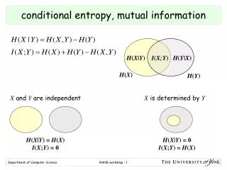
18. Joint and conditional entropy • Joint entropy is the entropy of the pairing (X,Y) • Conditional entropy is the entropy of X if the value of Y was known • Relationship between the two

19. Mutual information • Mutual information is how much information about X can be obtained by observing Y

20. Mathematical model of a channel • Assume that our input to the channel is X, and the output is Y • Then the characteristics of the channel can be defined by its conditional probability distribution p(y|x)

21. Channel capacity and rate • Channel capacity is defined as the maximum possible value of the mutual information • We choose the best f(x) to maximize C • For any rate R < C, we can transmit information with arbitrarily small probability of error

22. Binary symmetric channel • Correct bit transmitted with probability 1-p • Wrong bit transmitted with probability p • Sometimes called “cross-over probability” • Capacity C = 1 - H(p,1-p)

23. Binary erasure channel • Correct bit transmitted with probability 1-p • “Erasure” transmitted with probability p • Capacity C = 1 - p

24. Coding theory • Information theory only gives us an upper bound on communication rate • Need to use coding theory to find a practical method to achieve a high rate • 2 types • Source coding - Compress source data to a smaller size • Channel coding - Adds redundancy bits to make transmission across noisy channel more robust

25. Source-channel separation theorem • Shannon showed that when dealing with one transmitter and one receiver, we can break up source coding and channel coding into separate steps without loss of optimality • Does not apply when there are multiple transmitters and/or receivers • Need to use network information theory principles in those cases

26. Coding Intro • Assume alphabet K of{A, B, C, D, E, F, G, H} • In general, if we want to distinguish n different symbols, we will need to use, log2n bits per symbol, i.e. 3. • Can code alphabet K as:A 000 B 001 C 010 D 011 E 100 F 101 G 110 H 111

27. Coding Intro “BACADAEAFABBAAAGAH” is encoded as the string of 54 bits • 001000010000011000100000101000001001000000000110000111 (fixed length code)

28. Coding Intro • With this coding:A 0 B 100 C 1010 D 1011E 1100 F 1101 G 1110 H 1111 • 100010100101101100011010100100000111001111 • 42 bits, saves more than 20% in space

29. Huffman Tree A (8), B (3), C(1), D(1), E(1), F(1), G(1), H(1)

30. Huffman Encoding • Use probability distribution to determine how many bits to use for each symbol • higher-frequency assigned shorter codes • entropy-based, block-variable coding scheme

31. Huffman Encoding • Produces a code which uses a minimum number of bits to represent each symbol • cannot represent same sequence using fewer real bits per symbol when using code words • optimal when using code words, but this may differ slightly from the theoretical lower limit • lossless • Build Huffman tree to assign codes

32. Informal Problem Description • Given a set of symbols from an alphabet and their probability distribution • assumes distribution is known and stable • Find a prefix free binary code with minimum weighted path length • prefix free means no codeword is a prefix of any other codeword

33. Huffman Algorithm • Construct a binary tree of codes • leaf nodes represent symbols to encode • interior nodes represent cumulative probability • edges assigned 0 or 1 output code • Construct the tree bottom-up • connect the two nodes with the lowest probability until no more nodes to connect

34. Huffman Example • Construct the Huffman coding tree (in class)

35. Lowest probability symbol is always furthest from root Assignment of 0/1 to children edges arbitrary other solutions possible; lengths remain the same If two nodes have equal probability, can select any two Notes prefix free code O(nlgn) complexity Characteristics of Solution

36. Encode “BEAD” 001011011 Decode “0101100” Example Encoding/Decoding

37. Entropy (Theoretical Limit) = -.25 * log2 .25 + -.30 * log2 .30 + -.12 * log2 .12 + -.15 * log2 .15 + -.18 * log2 .18 H = 2.24 bits

38. Average Codeword Length = .25(2) +.30(2) +.12(3) +.15(3) +.18(2) L = 2.27 bits

39. Code Length Relative to Entropy • Huffman reaches entropy limit when all probabilities are negative powers of 2 • i.e., 1/2; 1/4; 1/8; 1/16; etc. • H <= Code Length <= H + 1

40. H = -.01*log2.01 + -.99*log2.99 = .08 L = .01(1) +.99(1) = 1 Example

41. Exercise • Compute Entropy (H) • Build Huffman tree • Compute averagecode length • Code “BCCADE”

42. Solution • Compute Entropy (H) • H = 2.1 bits • Build Huffman tree • Compute code length • L = 2.2 bits • Code “BCCADE” => 10000111101110

43. Limitations • Diverges from lower limit when probability of a particular symbol becomes high • always uses an integral number of bits • Must send code book with the data • lowers overall efficiency • Must determine frequency distribution • must remain stable over the data set

44. Error detection and correction • Error detection is the ability to detect errors that are made due to noise or other impairments during transmission from the transmitter to the receiver. • Error correction has the additional feature that enables localization of the errors and correcting them. • Error detection always precedes error correction. • (more next week)