Download
1 / 47
490 likes | 627 Views
Entropy and Information. For a random variable X with distribution p(x), entropy is given by H[ X ] = - S x p( x ) log 2 p( x ) “Information” = mutual information : how much knowing the value of one random variable r (the response)

E N D
Entropy and Information For a random variable X with distribution p(x), entropy is given by H[X] = - Sx p(x) log2p(x) “Information” = mutual information: how much knowing the value of one random variable r (the response) reduces uncertainty about another random variable s (the stimulus). Variability in response is due both to different stimuli and to noise. How much response variability is “useful”, i.e. can represent different messages, depends on the noise. Noise can be specific to a given stimulus. Need to know the conditional distribution P(s|r) or P(r|s). Take a particular stimulus s=s0 and repeat many times to obtain P(r|s0). Compute variability due to noise: noise entropy Information is the difference between the total response entropy and the mean noise entropy: I(s;r) = H[P(r)] – Ss P(s) H[P(r|s)] .
Information in single cells How can one compute the entropy and information of spike trains? Discretize the spike train into binary words w with letter size Dt, length T. This takes into account correlations between spikes on timescales TDt. Compute pi = p(wi), then the naïve entropy is Strong et al., 1997; Panzeri et al.
Information in single cells Many information calculations are limited by sampling: hard to determine P(w) and P(w|s) Systematic bias from undersampling. Correction for finite size effects: Strong et al., 1997
Information in single cells Information is the difference between the variability driven by stimuli and that due to noise. Take a stimulus sequence s and repeat many times. For each time in the repeated stimulus, get a set of words P(w|s(t)). Should average over all s with weight P(s); instead, average over time: Hnoise = < H[P(w|si)] >i. Choose length of repeated sequence long enough to sample the noise entropy adequately. Finally, do as a function of word length T and extrapolate to infinite T. Reinagel and Reid, ‘00
Information in single cells Obtain information rate of ~80 bits/sec or 1-2 bits/spike.
Information in single cells How much information does a single spike convey about the stimulus? Key idea: the information that a spike gives about the stimulus is the reduction in entropy between the distribution of spike times not knowing the stimulus, and the distribution of times knowing the stimulus. The response to an (arbitrary) stimulus sequence s is r(t). Without knowing that the stimulus was s, the probability of observing a spike in a given bin is proportional to , the mean rate, and the size of the bin. Consider a bin Dt small enough that it can only contain a single spike. Then in the bin at time t,
Now compute the entropy difference: prior conditional and using Assuming , In terms of information per spike (divide by ): Information in single cells , Note substitution of a time average for an average over the r ensemble.
Information in single cells Given • note that: • It doesn’t depend explicitly on the stimulus • The rate r does not have to mean rate of spikes; rate of any event. • Information is limited by spike precision, which blurs r(t), • and the mean spike rate. Compute as a function of Dt: Undersampled for small bins
Information in single cells An example: temporal coding in the LGN (Reinagel and Reid ‘00)
Information in single cells Apply the same procedure: collect word distributions for a random, then repeated stimulus.
Information in single cells Use this to quantify how precise the code is, and over what timescales correlations are important.
Information in single cells How important is information in multispike patterns? The information in any given event can be computed as: Define the synergy, the information gained from the joint symbol: or equivalently, Negative synergy is called redundancy. Brenner et al., ’00.
Information in single cells: multispike patterns In the identified neuron H1, compute information in a spike pair, separated by an interval dt: Brenner et al., ’00.
Information in single cells Information in patterns in the LGN Define pattern information as the difference between extrapolated word info and one letter: Reinagel and Reid ‘00
Using information to evaluate neural models We can use the information about the stimulus to evaluate our reduced dimensionality models.
Using information to evaluate neural models Information in timing of 1 spike: By definition
Given: By definition Bayes’ rule
So the information in the K-dimensional model is evaluated using the distribution of projections: Given: By definition Bayes’ rule Dimensionality reduction
Using information to evaluate neural models Here we used information to evaluate reduced models of the Hodgkin-Huxley neuron. Twist model 2D: two covariance modes 1D: STA only
Adaptive coding • Just about every neuron adapts. Why? • To stop the brain from pooping out • To make better use of a limited • dynamic range. • To stop reporting already known facts • All reasonable ideas. • What does that mean for coding? • What part of the signal is the brain meant • to read? • Adaptation can be mechanism for early • sensory systems to make use of statistical • Information about the environment. • How can the brain interpret an adaptive • code? From The Basis of Sensation, Adrian (1929)
Adaptation to stimulus statistics: information Rate, or spike frequency adaptation is a classic form of adaptation. Let’s go back to the picture of neural computation we discussed before: Can adapt both: the system’s filters the input/output relation (threshold function) Both are observed, and in both cases, the observed adaptations can be thought of as increasing information transmission through the system. Information maximization as a principle of adaptive coding: For optimum information transmission, coding strategy should adjust to the statistics of the inputs. To compute the best strategy, have to impose constraints (Stemmler&Koch) e.g. the variance of the output, or the maximum firing rate.
Adaptation of the input/output relation If we constrain the maximum, the solution for the distribution of output symbols is P(r) = constant = a. Take the output to be a nonlinear transformation on the input: r = g(s). From Fly LMC cells. Measured contrast in natural scenes. Laughlin ’81.
Adaptation of filters Change in retinal filters with different light level and contrast Changes in V1 receptive fields with contrast
Smirnakis et al., ‘97 Dynamical adaptive coding But is all adaptation to statistics on an evolutionary scale? The world is highly fluctuating. Light intensities vary by 1010 over a day. Expect adaptation to statistics to happen dynamically, in real time. Retina: observe adaptation to variance, or contrast, over 10s of seconds. Surprisingly slow: contrast gain control effects after 100s of milliseconds. Also observed adaptation to spatial scale on a similar timescale.
Dynamical adaptive coding The H1 neuron of the fly visual system. Rescales input/output relation with steady state stimulus statistics. Brenner et al., ‘00
Dynamical adaptive coding As in the Smirnakis et al. paper, there is rate adaptation in response to the variance change
Dynamical adaptive coding This is a form of learning. Does the timescale reflect the time required to learn the new statistics?
Dynamical adaptive coding As we have been through before, extract the spike-triggered average
Dynamical adaptive coding Compute the input/output relations, as we described before: s = stim . STA; P(spike|s) = rave P(stim|s) / P(s) Do it at different times in variance modulation cycle. Find ongoing normalisation with respect to stimulus standard deviation
Dynamical adaptive coding Take a more complex stimulus: randomly modulated white noise. Not unlike natural stimuli (Ruderman and Bialek ’97)
Find continuous rescaling to variance envelope.
Dynamical information maximisation This should imply that information transmission is being maximized. We can compute the information directly and observe the timescale. How much information is available about the stimulus fluctuations? Return to two-state switching experiment. Method: Present n different white noise sequences, randomly ordered, throughout the variance modulation. Collect word responses indexed by time with respect to the cycle, P(w(t)). Now divide according to probe identity, and compute It(w;s) = H[P(w(t))] – Si P(si) H[P(w(t)|si)] , P(si) = 1/n; Similarly, one can compute information about the variance: It(w;s) = H[P(w(t))] – Si P(si) H[P(w(t)|si)] , P(si) = ½; Convert to information/spike by dividing at each time by mean # of spikes.
Adaptation and ambiguity The stimulus normalization is leading to information recovery within 100ms. If the stimulus is represented as normalised, how are the spikes to be interpreted upstream? The rate conveys variance information, but with slow timescales.
What conveys variance information? Where is the variance information and how can one decode it? Notice that the interspike interval histograms in the different variance regimes are quite distinct. Need to take log to see this clearly. Could these intervals provide enough information, rapidly, to distinguish the variance?
Decoding the variance information Use signal detection theory. Collect the steady-state distributions: P(d|si). Then for a given observation, compute the likelihood ratio, P(d|s1)/P(d|s2). After observing a sequence of intervals, compute the log-likelihood ratio for the entire sequence Since we can’t sample the joint distributions, we will assume that the intervals are independent (upper bound). Now calculate the signal to noise ratio of Dn, <Dn>2/var(Dn), as a function of n.
Decoding the variance information On average, the number of intervals required for accurate discrimination is ~5-8.
Adaptive coding: conclusions Have shown that information is available from the spike train in three forms: timing of single spikes the rate the local distribution of spike intervals. The adaptation properties in some systems serve to rapidly maximize information transmission through the system under conditions of changing stimulus statistics. We demonstrated this for the variance: in other systems can probe adaptation to more complex stimulus correlations (Meister) Mechanisms remain open: intrinsic properties conductance level learning (Tony,Stemmler&Koch, Turrigiano) circuit level learning (Tony)
Conclusions Characterising the neural computation: uncovering the richness of single neurons and systems Using information to evaluate coding Adaptation as a method for the brain to make use of stimulus statistics more examples? how is it implemented?
Cockroach leg mechanoreceptor, to spinal distortion • Spider slit sensillum, to 1200 Hz sound • Stretch receptor of the crayfish • Limulus eccentric-cell, to increase in light intensity Thorson and Biederman-Thorson, Science (1974) The rate dynamics: what’s going on • Recall: no fixed timescale • Consistent with • power-law adaptation Suggests that rate behaves like fractional differentiation of the log-variance envelope
Fractional differentiation scaling “adaptive” response to a square wave: power-law response to a step: Fourier representation (iw)a : each frequency component scaled by wa and with phase shifted by a constant phase ia ap
phase shift T = 30s, 60s, 90s Linear analysis agrees • Stimulate with a set of sine waves • at different frequencies • Variance envelope ~ exp[sin t/T] • for a range of frequencies 1/T
Three-state switching Two-state switching Fits pretty well From sinusoid experiments, find exponent a ~ 0.2
So it’s a fractional differentiator… • connects with “universal” power-law behaviour of receptors • uncommon to see it in a “higher computation” • functional interpretation: whitening stimulus spectrum • (van Hateren) • introduces long history dependence: • linear realisation of long memory effects • also has the property of emphasizing rapid changes and • extending dynamic range (Adrian) • but what’s the mechanism? --- some ideas but we don’t know