Download
1 / 89
890 likes | 907 Views
Choosing the Optimal Sequences and Strategies for Functional MRI. Peter A. Bandettini, Ph.D Unit on Functional Imaging Methods Laboratory of Brain and Cognition National Institute of Mental Health. Variables to Optimize. Information Content Sensitivity Speed Resolution Image quality.

E N D
Choosing the Optimal Sequences and Strategies for Functional MRI Peter A. Bandettini, Ph.D Unit on Functional Imaging Methods Laboratory of Brain and Cognition National Institute of Mental Health
Variables to Optimize • Information Content • Sensitivity • Speed • Resolution • Image quality
Variables to Optimize • Information Content • Sensitivity • Speed • Resolution • Image quality
Information Content • Blood Volume • Blood Oxygenation • Blood Perfusion • Hemodynamic Specificity • Mapping of CMRO2
Blood Volume Contrast agent injection and time series collection of T2* or T2 - weighted images
BOLD Contrast in the Detection of Neuronal Activity Cerebral Tissue Activation Local Vasodilation Oxygen Delivery Exceeds Metabolic Need Increase in Cerebral Blood Flow and Volume Increase in Capillary and Venous Blood Oxygenation Deoxy-hemoglobin: paramagnetic Oxy-hemoglobin: diamagnetic Decrease in Deoxy-hemoglobin Decrease in susceptibility-related intravoxel dephasing Increase in T2 and T2* Local Signal Increase in T2 and T2* - weighted sequences
The BOLD Signal Blood Oxygenation Level Dependent (BOLD) signal changes task task
Blood Perfusion EPISTAR FAIR . . . - - - - Perfusion Time Series . . .
TI (ms) 200 400 600 800 1000 1200 FAIR EPISTAR
Perfusion Rest Activation BOLD
Anatomy BOLD Perfusion
+- • unique information • baseline information • multislice trivial • invasive • low C / N for func. Volume BOLD Perfusion • highest C / N • easy to implement • multislice trivial • non invasive • highest temp. res. • complicated signal • no baseline info. • unique information • control over ves. size • baseline information • non invasive • multislice non trivial • lower temp. res. • low C / N
Hemodynamic Specificity Arterial inflow (BOLD TR < 500 ms) Venous inflow (Perf. No VN)
Mapping of CMRO2 Activation: Flow CMRO2 Blood Oxygenation CO2 stress: Flow CMRO2 Blood Oxygenation
20 3 15 2 10 BOLD (% increase) CBF (% increase) 5 1 0 0 -5 -10 0 200 400 600 800 1000 1200 1400 0 200 400 600 800 1000 1200 1400 Time (seconds) Time (seconds) hypercapnia visual stimulation Hoge, et al. CMRO2-related BOLD signal deficit: CBF BOLD Simultaneous Perfusion and BOLD imaging during graded visual activation and hypercapnia N=12
4 +10 +20 -10 0 25 3 20 15 CMRO2 (% increase) BOLD (% increase) 2 10 5 1 0 0 10 20 30 40 50 Perfusion (% increase) 0 0 10 20 30 40 50 Perfusion (% increase) Hoge, et al. CBF-CMRO2 coupling Characterizing Activation-induced CMRO2 changes using calibration with hypercapnia
Hoge, et al. Computed CMRO2 Changes 40 30 20 10 0 % % -10 -20 -30 -40 Subject 2 Subject 1
Variables to Optimize • Information Content • Sensitivity • Speed • Resolution • Image quality
Sensitivity • Optimizing fMRI Contrast • Maximizing Signal • Reducing Physiologic Fluctuations • Minimizing Temporal Artifacts
Optimizing fMRI Contrast • Increase field strength • Adjust pulse sequence timing (TE ≈ T2*) • Adjust voxel volume (≈ activation volume)
Asymmetric Spin - Echo Gradient - Echo
Asymmetric Spin - Echo Gradient - Echo
Asymmetric Spin - Echo Gradient - Echo
Maximizing Signal • Higher Bo Field • Radio frequency Coils • Choice of repetition time (TR) • Voxel volume
Physiologic Fluctuations Cardiac 0.6 to 1.2 Hz Respiratory 0.1 to 0.2 Hz Low Frequency 0.0 to 0.1 Hz
0.25 Hz Breathing at 1.5T 3ms 3ms Image 26ms Power Spectra Respiration map 49ms 0 0.25 0.5 Hz
0.68 Hz Cardiac rate at 3T 3ms Image 26ms Power Spectra Cardiac map 49ms 0 0.68 (aliased) 0.5 Hz
Temporal vs. Spatial SNR- 3T 26ms 49ms 26ms 49ms SPIRAL 27ms 50ms 27ms 50ms EPI
Reducing Physiologic Fluctuations • Filtering • Pulse sequence • single vs. multishot • strategies for multishot • Gating with correction for variable TR
Temporal Artifacts • System instabilities • Motion • Drift • Stimulus correlated • Stimulus uncorrelated
Minimizing Temporal Artifacts • Recognize? • Edge effects • Shorter signal change latencies • Unusually high signal changes • External measuring devices • Correct? • Image registration algorithms • Orthogonalize to motion-related function (cardiac, respiration, movement) • Navigator echo for k-space alignment (for multishot techniques) • Re-do scan • Bypass? • Paradigm timing strategies.. • Gating (with T1-correction) • Suppress? • Flatten image contrast • Physical restraint • Averaging, smoothing
Overt Word Production 2 3 4 5 6 7 8 9 10 11 12 13
Tongue Movement Jaw Clenching
Variables to Optimize • Information Content • Sensitivity • Speed • Resolution • Image quality
Speed • Rapid imaging techniques: • Single shot imaging • TR vs. Brain coverage: min TR = (time/slice) x number of slices in volume • Hemodynamic Issues • Paradigm timing • Event related fMRI • Timing modulation
Single Shot Imaging T2* decay EPI Readout Window ≈ 20 to 40 ms
2 1000 msec 1.5 100 msec 34 msec 1 0.5 0 -0.5 -1 15 20 25 30 35 Time (sec)
a t Compute nonlinearity (for each voxel) • Amplitude of Response Fit ideal (linear) to response • Area under response / Stimulus Duration Output Area / Input Area
6 6 4 f (SD) 4 f (SD) 2 2 0 1 2 3 4 5 0 1 2 3 4 5 Stimulus Duration Stimulus Duration 6 5 4 4 3 2 2 1 0 1 2 3 4 5 0 1 2 3 4 5 Nonlinearity Visual Motor Magnitude linear Area Output / input Output / input Stimulus Duration Stimulus Duration
Results – visual task Nonlinearity Magnitude Latency
Results – motor task Nonlinearity Magnitude Latency