Download
1 / 93
940 likes | 1.34k Views
Solving LP Models. Improving Search Unimodal Convex feasible region Should be successful! Special Form of Improving Search Simplex method (now) Interior point methods (later). Simple Example. Top Brass Trophy Company Makes trophies for football

E N D
Solving LP Models • Improving Search • Unimodal • Convex feasible region • Should be successful! • Special Form of Improving Search • Simplex method (now) • Interior point methods (later) IE 312
Simple Example • Top Brass Trophy Company • Makes trophies for • football • wood base, engraved plaque, brass football on top • $12 profit and uses 4’ of wood • soccer • wood base, engraved plaque, soccer ball on top • $9 profit and uses 2’ of wood • Current stock • 1000 footballs, 1500 soccer balls, 1750 plaques, and 4800 feet of wood IE 312
Formulation IE 312
2000 1500 1000 500 500 1000 1500 2000 Graphical Solution Optimal Solution IE 312
Feasible Solutions • Feasible solution is a • boundary point if at least one inequality constraint that can be strict is active • interior point if no such constraints are active • Extreme points of convex sets do not lie within the line segment of any other points in the set IE 312
2000 1500 1000 500 500 1000 1500 2000 Example IE 312
Optimal Solutions • Every optimal solution is a boundary point • We can find an improving direction whenever we are at an interior point • If optimum unique the it must be an extreme point of the feasible region • If optimal solution exist, an optimal extreme point exists IE 312
LP Standard Form • Easier if we agree on exactly what a LP should look like • Standard form • only equality main constraints • only nonnegative variables • variables appear at most once in left-hand-side and objective function • all constants appear on right hand side IE 312
Converting to Standard • Inequality constraints • Add nonnegative, zero-cost slack variables • Add in inequalities • Subtract in inequalities • Variables not nonnegative • nonpositive - substitute with negatives • unrestrictive sign (URS) - substitute difference of two nonnegative variables IE 312
Top Brass Model IE 312
Why? • Feasible directions • Check only if active • Keep track of active constraints • Equality constraints • Always active • Inequality constraints • May or may not be active • Prefer equality constraints! IE 312
Standard Notation IE 312
LP Standard Form • In standard notation • In matrix notation IE 312
Write in Matrix Form IE 312
Extreme Points • Know that an extreme point optimum exists • Will search trough extreme points • An extreme point is define by a set of constraints that are active simultaneously IE 312
Improving Search • Move from one extreme point to a neighboring extreme point • Extreme points are adjacent if they are defined by sets of active constraints that differ by only one element • An edge is a line segment determined by a set of active constraints IE 312
Basic Solutions • Extreme points are defined by set of active nonnegativity constraints • A basic solution is a solution that is obtained by fixing enough variable to be equal to zero, so that the equality constraints have a unique solution IE 312
Example Choose x1, x2, x3, x4 to be basic IE 312
2000 1500 1000 500 500 1000 1500 2000 Where is the Basic Solution? IE 312
Example • Compute the basic solution for x1 and x2 basis: • Solve IE 312
Existence of Basis Solutions • Remember linear algebra? • A basis solution exists if and only if the columns of corresponding equality constraint form a basis (in other words, a largest possible linearly independent collection) IE 312
Checking • The determinant of a square matrix D is • A matrix is singular if its determinant = 0 and otherwise nonsingular • Need to check that the matrix is nonsingular IE 312
Example • Check whether basic solutions exist for IE 312
Basic Feasible Solutions • A basic feasible solution to a LP is a basic solution that satisfies all the nonnegativity contraints • The basic feasible solutions correspond exactly to the extreme points of the feasible region IE 312
Example Problem • Suppose we have x3, x4, x5 as slack variables in the following LP: • Lets plot the original problem, compute the basic solutions and check feasibility IE 312
Solution Algorithm • Simplex Algorithm • Variant of improving search • Standard display: IE 312
Simplex Algorithm • Starting point • A basic feasible solution (extreme point) • Direction • Follow an edge to adjacent extreme point: • Increase one nonbasic variable • Compute changes needed to preserve equality constraints • One direction for each nonbasic variable IE 312
Top Brass Example Basic variables Initial solution IE 312
Looking in All Directions … Can increase either one of those Must adjust these! IE 312
So Many Choices ... • Want to try to improve the objective • The reduced cost of a nonbasic variable: • Want Defines improving direction IE 312
Top Brass Example • Improving x1 gives • Improving x2 gives • Both directions are improving directions! IE 312
Where and How Far? • Any improving direction will do • If no component is negative Improve forever - unbounded! • Otherwise, compute the minimum ratio IE 312
Computing Minimum Ratio IE 312
Moving to New Solution IE 312
Updating Basis • New basic variable • Nonbasic variable generating direction • New nonbasic variable(s) • Basic variables fixing the step size IE 312
2000 1500 1000 500 500 1000 1500 2000 What Did We Do? IE 312
2000 1500 1000 500 500 1000 1500 2000 Where Will We Go? Optimum in three steps! Why is this guaranteed? IE 312
Simplex Algorithm (Simple) Step 0: Initialization. Choose starting feasible basis, construct basic solution x(0), and set t=0 Step 1: Simplex Directions. Construct directions Dx associated with increasing each nonbasic variable xj and compute the reduced cost cj =c ·Dx. Step 2: Optimality. If no direction is improving, then stop; otherwise choose any direction Dx(t+1) corresponding to some basic variable xp. Step 3: Step Size. If no limit on move in direction Dx(t+1) then stop; otherwise choose variable xr such that Step 4: New Point and Basis. Compute the new solution and replace xr in the basis with xp. Let t = t+1 and go to Step 1. IE 312
Stopping • The algorithm stop when one of two criteria is met: • In Step 2 if no improving direction exists, which implies local optimum, which implied global optimum • In Step 3 if no limit on improvement, which implies problem is unbounded IE 312
Optimization Software • Spreadsheet (e.g, MS Excel with What’s Best!) • Optimizers (e.g., LINDO) • Combination • Modeling Language • Solvers • Either together (e.g., LINGO) or separate (e.g., GAMS with CPLEX) • LINDO and LINGO are in Room 0010 (OR Lab) • Also on disk with your book IE 312
LINDO • The main software that I’ll ask you to use is called LINDO • Solves linear programs (LP), integer programs (IP), and quadratic programs (QP) • We will look at many of its more advanced features later on, but as of yet we haven’t learned many of the concepts that we need IE 312
Example IE 312
LINDO Program MAX 12 x1 + 9 x2 ST x1 + x2 = 1000 x2 + x4 = 1500 x1 + x2 + x5 = 1750 4x1+ 2x2 + x6 = 4800 x1>=0 x2>=0 x3>=0 x4>=0 x5>=0 x6>=0 END IE 312
Output LP OPTIMUM FOUND AT STEP 4 OBJECTIVE FUNCTION VALUE 1) 12000.00 VARIABLE VALUE REDUCED COST X1 1000.000000 0.000000 X2 0.000000 3.000000 X4 1500.000000 0.000000 X5 750.000000 0.000000 X6 800.000000 0.000000 X3 0.000000 0.000000 IE 312
Output (cont.) ROW SLACK OR SURPLUS DUAL PRICES 2) 0.000000 12.000000 3) 0.000000 0.000000 4) 0.000000 0.000000 5) 0.000000 0.000000 6) 1000.000000 0.000000 7) 0.000000 0.000000 8) 0.000000 0.000000 9) 1500.000000 0.000000 10) 750.000000 0.000000 11) 800.000000 0.000000 NO. ITERATIONS= 4 IE 312
LINDO: Basic Syntax • Objective Function Syntax: Start all models with MAX or MIN • Variable Names: Limited to 8 characters • Constraint Name: Terminated with a parenthesis • Recognized Operators (+, -, >, <, =) • Order of Precedence: Parentheses not recognized IE 312
Syntax (cont.) • Adding Comment: Start with an exclamation mark • Splitting lines in a model: Permitted in LINDO • Case Sensitivity: LINDO has none • Right-hand Side Syntax: Only constant values • Left-hand Side Syntax: Only variables and their coefficients IE 312
Why Modeling Language? • More to learn! • More ‘complicated’ to use than LINDO (at least at first glance) • Advantages • Natural representations • Similar to mathematical notation • Can enter many terms simultaneously • Much faster and easier to read IE 312