Download
1 / 45
450 likes | 519 Views
Learn how to utilize Excel's Solver tool for solving linear programming problems efficiently. Follow step-by-step instructions on setting up LP models in Excel, enabling Solver, and implementing constraints. This guide provides clear explanations and visual examples to help you master LP problem-solving in spreadsheets.

E N D
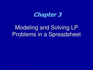
Chapter 3 Modeling and Solving LP Problems in a Spreadsheet
Introduction • Solving LP problems graphically is only possible when there are two decision variables. • Few real-world LP have only two decision variables. • Fortunately, we can now use spreadsheets (i.e., Excel’s Solver) to solve LP problems.
Spreadsheet Solvers • We will be using Excel’s Solver to solve linear programming problems. • You access Solver from Excel’s Data tool bar menu. • If Solver is not present, click on the Office button (in Excel 2007) or File button (in Excel 2010), then Excel Options, followed by Add-ins, then click on “Go” at the bottom of the window to manage Excel’s add-ins, and finally make sure that the check box for Solver add-In is enabled. The next slides provide you with screen shots of enabling Solver if it is not present.
Enabling Solver: Step 1Excel 2007 Step 1: Click here
Enabling Solver: Step 2 Step 2:Click on Excel Options, then “Add-Ins”
Enabling Solver: Step 3 Step 3: Click on “Go”
Enabling Solver: Step 4 Step 4: Check the Solver Add-In box
Solver for MAC Those of you who have a MAC can still download Solver for Macintosh Excel 2008. It’s free and can be downloaded by following the instructions provided in the following link (copy and paste into your browswer): http://www.solver.com/mac/dwnmacsolver.htm
Solver (continued) • Note: there is no need to install Premium Solver for Education (see pp. 53 of your textbook), as the standard Solver that is within Excel is capable of solving all problems. • The Simplex method is the default algorithm that the standard version of Excel’s Solver uses in solving LP problems.
Steps in Implementing an LP Model in a Spreadsheet 1. Organize the data for the model in the spreadsheet. 2. Reserve separate cells in the spreadsheet for each decision variable in the model. 3. Create a formula in a cell in the spreadsheet that corresponds to the objective function. 4. For each constraint, create a formula in a separate cell in the spreadsheet that corresponds to the left-hand side (LHS) of the constraint.
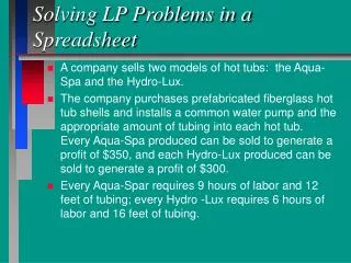
Let’s Implement a Model for the Blue Ridge Hot Tubs Example... MAX: 350X1 + 300X2 } profit S.T.: 1X1 + 1X2 <= 200 } pumps 9X1 + 6X2 <= 1566 } labor 12X1 + 16X2 <= 2880 } tubing X1, X2 >= 0 } nonnegativity
Using Solver Please note that there two steps to solve any type of a linear programming problem: Step 1: Set the problem up in a spreadsheet. Step 2: Invoke Solver to enter all pertinent parameters. The next slide shows the first step which entails setting the problem up in Excel.
Using Solver Let’s break up the spreadsheet set up into smaller pieces so that we do not find it overwhelming. Please note that I’ll explain the set up in a more generic way before going into specifics.
Step 1: Designate an Area for the Optimal Solution We reserve any area in the spreadsheet for the optimal solution
Step 2: Create an Equation for the Objective Function The equation will be created in this cell
Step 3: Input Each Constraint’s Coefficients Pump constraint is: 1X1 +1X2 <= 200, so we input the values 1 and 1 in row 9 to reflect the coefficients of this constraint. Same approach for the other constraints.
Step 4: Create an Equation for Each Constraint’s L.H.S. Each L.H.S. reflects consumption of resources. We will worry about the equation itself later on.
Step 6: Creating the Equations B6*B5+C6*C5 B9*B5+C9*C5 B10*B5+C10*C5 B11*B5+C11*C5
Solver Parameters Objective Function Equation Cell Reserved Cells for Optimal Solution R.H.S. of Constraints L.H.S. of Constraints
How Solver Views the Model • Target cell - the cell in the spreadsheet that represents the objective function • Changing cells - the cells in the spreadsheet representing the decision variables • Constraint cells - the cells in the spreadsheet representing the LHS formulas on the constraints
Implementing the Model Week 2 Multimedia contains a link to an Excel file called Fig3-1.xls. Please open the file to view it. Note: the first worksheet in Fig3-1.xls,called “model”, illustrates the set up of the problem in Excel along with all the pertinent equations. The second worksheet, “solution”, illustrates the optimal solution to the problem using Solver. See pp. 48-60 of your textbook for full details.
Solver (continued) • Do not forget to always specify the linearity and non-negativity assumptions in Solver. • This can be accomplished by checking the check boxes Assume Non-Negative and Assume Linear Model in the Solver Options dialog box.
Video Clips • Please view the video clips Sumproduct Function and Solver Example.
Model 1 Model 2 Model 3 Number ordered 3,000 2,000 900 Hours of wiring/unit 2 1.5 3 Hours of harnessing/unit 1 2 1 Cost to Make $50 $83 $130 Cost to Buy $61 $97 $145 Make vs. Buy Decisions:The Electro-Poly Corporation • Electro-Poly is a leading maker of slip-rings. • A $750,000 order has just been received. • The company has 10,000 hours of wiring capacity and 5,000 hours of harnessing capacity.
Defining the Decision Variables M1 = Number of model 1 slip rings to make in-house M2 = Number of model 2 slip rings to make in-house M3 = Number of model 3 slip rings to make in-house B1 = Number of model 1 slip rings to buy from competitor B2 = Number of model 2 slip rings to buy from competitor B3 = Number of model 3 slip rings to buy from competitor
Defining the Objective Function Minimize the total cost of filling the order. MIN: 50M1+ 83M2+ 130M3+ 61B1+ 97B2+ 145B3
Defining the Constraints • Demand Constraints M1 + B1 = 3,000 } model 1 M2 + B2 = 2,000 } model 2 M3 + B3 = 900 } model 3 • Resource Constraints 2M1 + 1.5M2 + 3M3 <= 10,000 } wiring 1M1 + 2.0M2 + 1M3 <= 5,000 } harnessing • Nonnegativity Conditions M1, M2, M3, B1, B2, B3 >= 0
Implementing the Model See file Fig3-17.xls See pp. 63-67 of your textbook for full details.
Years to Company Return Maturity Rating Acme Chemical 8.65% 11 1-Excellent DynaStar 9.50% 10 3-Good Eagle Vision 10.00% 6 4-Fair Micro Modeling 8.75% 10 1-Excellent OptiPro 9.25% 7 3-Good Sabre Systems 9.00% 13 2-Very Good An Investment Problem:Retirement Planning Services, Inc. • A client wishes to invest $750,000 in the following bonds.
Investment Restrictions • No more than 25% can be invested in any single company. • At least 50% should be invested in long-term bonds (maturing in 10+ years). • No more than 35% can be invested in DynaStar, Eagle Vision, and OptiPro.
Defining the Decision Variables X1 = amount of money to invest in Acme Chemical X2 = amount of money to invest in DynaStar X3 = amount of money to invest in Eagle Vision X4 = amount of money to invest in MicroModeling X5 = amount of money to invest in OptiPro X6 = amount of money to invest in Sabre Systems
Defining the Objective Function Maximize the total annual investment return: MAX: .0865X1+ .095X2+ .10X3+ .0875X4+ .0925X5+ .09X6
Defining the Constraints • Total amount invested X1 + X2 + X3 + X4 + X5 + X6 = 750,000 • No more than 25% in any one investment Xi <= 187,500, for all i • 50% long term investment restriction. X1 + X2 + X4 + X6 >= 375,000 • 35% Restriction on DynaStar, Eagle Vision, and OptiPro. X2 + X3 + X5 <= 262,500 • Nonnegativity conditions Xi >= 0 for all i
Implementing the Model See file Fig3-20.xls Also see pp. 67-71 of your textbook for full details. Please note that I have prepared a video clip of this problem for you to view. The problem is set up in a more classic and traditional way than the author’s approach. So, please view it under the title “The Investment Problem”.
Processing Plants Groves Distances (in miles) Supply Capacity 21 Mt. Dora Ocala 200,000 275,000 1 4 50 40 35 30 Eustis Orlando 600,000 400,000 2 5 22 55 20 Clermont Leesburg 225,000 300,000 3 6 25 A Transportation Problem: Tropicsun
Defining the Decision Variables Xij= # of bushels shipped from node ito node j Specifically, the nine decision variables are: X14 = # of bushels shipped from Mt. Dora (node 1) to Ocala (node 4) X15 = # of bushels shipped from Mt. Dora (node 1) to Orlando (node 5) X16 = # of bushels shipped from Mt. Dora (node 1) to Leesburg (node 6) X24 = # of bushels shipped from Eustis (node 2) to Ocala (node 4) X25 = # of bushels shipped from Eustis (node 2) to Orlando (node 5) X26 = # of bushels shipped from Eustis (node 2) to Leesburg (node 6) X34 = # of bushels shipped from Clermont (node 3) to Ocala (node 4) X35 = # of bushels shipped from Clermont (node 3) to Orlando (node 5) X36 = # of bushels shipped from Clermont (node 3) to Leesburg (node 6)
Defining the Objective Function Minimize the total number of bushel-miles. MIN: 21X14 + 50X15 + 40X16 + 35X24 + 30X25 + 22X26 + 55X34 + 20X35 + 25X36
Defining the Constraints • Capacity constraints X14 + X24 + X34 <= 200,000 } Ocala X15 + X25 + X35 <= 600,000 } Orlando X16 + X26 + X36 <= 225,000 } Leesburg • Supply constraints X14 + X15 + X16 = 275,000 } Mt. Dora X24+ X25 + X26 = 400,000 } Eustis X34 + X35 + X36 = 300,000 } Clermont • Nonnegativity conditions Xij>= 0 for all iandj
Implementing the Model See file Fig3-24.xls Note that spreadsheet Fig3-24.xls contains the model with all the pertinent formulas. You need to invoke Solver and specify your Target Cell, Changing Cells and constraints to get the optimal solution. See pp. 72-78 for full details.
Transportation Problem (continued) General guidelines in formulating the transportation problem: • When total supply = total demand, all supply constraints will have equality signs and all demand constraints will have equality signs. • When total supply < total demand, all demand constraints will have “<=“ signs and all supply constraints will have “>=“ signs. • When total supply > total demand, all supply constraints will have “<=“ signs and all demand constraints will have “>=“ signs.
Video Clip • Please view the video clip “The Transportation Problem” which will provide you with a nice overview of how to set up and solve a classic transportation problem using Solver.