Download
1 / 14
140 likes | 192 Views
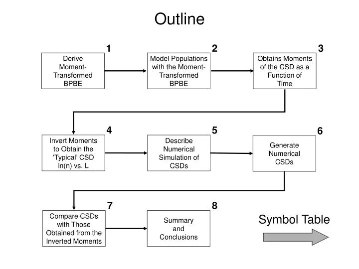
Model Populations with the Moment- Transformed BPBE. Describe Numerical Simulation of CSDs. Derive Moment- Transformed BPBE. Obtains Moments of the CSD as a Function of Time. Compare CSDs with Those Obtained from the Inverted Moments. Invert Moments to Obtain the

E N D
Model Populations with the Moment- Transformed BPBE Describe Numerical Simulation of CSDs Derive Moment- Transformed BPBE Obtains Moments of the CSD as a Function of Time Compare CSDs with Those Obtained from the Inverted Moments Invert Moments to Obtain the ‘Typical’ CSD ln(n) vs. L Generate Numerical CSDs Summary and Conclusions Symbol Table Outline 1 2 3 4 5 6 7 8
The Batch Population Balance Equation (BPBE) is: Here, nucleation is included as a source term and the derivation of Hulburt and Katz (1964) is followed. The moments of a crystal size distribution (CSD) are calculated as follows (see also, e.g., Randolph and Larson, 1988): This transformation is applied to the BPBE:
For the third term, assume: This gives: The integration is applied to each term of the BPBE. First term: For the second term, assume G G(L). Integration by parts gives:
...but, since mj = mj(t): j = 1, 2, 3,... Assembling terms yields the moment-transformed BPBE: Thus, a single partial differential equation (the BPBE) may now be represented by a set of ordinary differential equations (ODEs). Now, let crystal growth rate, G, be given by: The crystal nucleation rate, I, is given by Cashman (1993):
(cooling rate of the liquid ...with latent heat) Now: where L0 = 0.5 x 10⁻⁶ m The cooling rate is from Jaeger (1957) for an infinite half-sheet of magma: This combination of G and I mechanisms has been demonstrated to yield CSDs typical of those in natural rocks (Resmini, 2001; 2002). This now yields the following set of ODEs (for j = 0 to 7; see below):
(Implicit in derivation of cooling rate expression.) This is a set of nonlinear ordinary differential equations (ODEs) solvable numerically using a fourth-order Runge-Kutta method. Though the set of ODEs is closed after j = 2, eight equations are utilized to facilitate an inversion of the moments. The solution to the set of ODEs is a table of eight moment values as a function of time (from first nucleation event to complete solidification).
Moments … … … … … … … … … For a position located one meter from the contact within the infinite half-sheet described by the Jaeger (1957) cooling-rate expression, the moments are as follows: Complete solidification at x’ = 1 meter after 457 hours
The set of eight moment values may be inverted to yield the more familiar crystal size distribution plot; i.e., ln(n) vs. L. This is done using constrained linear inversion according to the following equation: where: n(L) is the crystal population density as a function of crystal size; K is a matrix of quadrature coefficients (aka kernel function); g is a Lagrange multiplier; H is a smoothing matrix of 2nd order finite-difference coefficients; and mj* is a vector of the first eight moments (calculated above) K is calculated with a weighting function to smooth n(L) vs. L Constrained linear inversion as applied here is described in, e.g., Twomey (1977), Steele and Turco (1997) and King (1982).
and is a smoothing matrix. n(L) is obtained by multiplying by h(L) after inversion: For brevity, the terms for the inversion are shown, below, for four moments: The matrix on the left is K and is derived from a quadrature approximation to the integral equation that defines the moments of the crystal population. h(L) is a weighting function to smooth n(L). La - Ld represent four crystal sizes. The right-most vector is mj*. The ‘usual’ CSD is generated by computing ln(n(L)) and plotting vs. L.
Moment 25 20 From Resmini (2001) 15 ln(n), no./cm4 10 5 From the inversion 0 0.00 0.01 0.02 0.03 0.04 0.05 0.06 L (cm) The first four moments are compared to those obtained from the model of Resmini (2001) for 100% solidification. Agreement is excellent. Both CSDs are typical of those observed in natural rocks. The CSD is compared to one obtained from the model of Resmini (2001).
Summary and Conclusions • A moment transformation is applied to the batch population balance equation(BPBE), a number continuity equation describing the evolution of crystalpopulations in closed magmatic systems such as sills. • The more typical CSD, usually presented as a plot of the natural log ofcrystal population density (ln(n)) vs. crystal size (L), is obtained by inversionof the moments. • The CSDs recovered by constrained linear inversion of the momentsare similar to those observed in natural rocks. • The moments of the crystal population are, to within ~0.4%, identical to thosegenerated by the numerical simulation described in Resmini (2001). • These results demonstrate an equivalence between equation-based modelingand a numerical simulation of evolving crystal populations. • Modeling crystal populations with the moment-transformed BPBE is faster thanthe iterative, computationally-intensive simulation of Resmini (2001).
Acknowledgements Partial funding for this work provided by The Boeing Company. References Cited